CVAE
Sohn, Kihyuk, Honglak Lee, and Xinchen Yan. “Learning structured output representation using deep conditional generative models.” Advances in neural information processing systems 28 (2015). citations:2250
http://ijdykeman.github.io/ml/2016/12/21/cvae.html (翻译:https://www.cnblogs.com/sddai/p/10523431.html)
思路
提出一种生成模型的训练方法,该模型在随机梯度变分 Bayes框架下进行有效训练,此外,我们提供了新的策略来构建robust的结构化预测 算法,是一个深度条件 生成模型,用于使用高斯潜变量进行结构化输出预测。例如在 训练中输入噪声注入和多尺度预测目标。
structured output 我理解的是多种特征、属性都有一点的结构化输出
multi-modal distribution 我理解就是组成output分布的多种特征、属性,多种特征的分布组成了多模态分布
在分割精度、条件对数似然估计和生成样本的可视化方面表现出色
对生成模型(或者说预测任务)的要求有两个:1.可以形成好的概率分布probabilistic inference(生成的样本和训练样本的分布是接近的);2. 可以生成出不一样的样本,不能生成出来的样本都很接近,要是不一样的。
提出conditional variational auto-encoder (CVAE).CVAE是一个有条件的 有向图模型(z生成x,有个方向),其输入观测调节了产生输出的高斯潜变量 的先验 p(z)
主要改进如下:
- 提出了cvae,我们提出了CVAE及其在SGVB框架中可有效训练的变体, ,并引入了新的策略来增强结构化预测模型的鲁棒性。
- 我们用高斯随机神经元 证明了我们提出的算法在建模结构化输出变量的多模态分布方面的有效性
- 我们在CUB和LFW数据集上实现了强大的语义对象分割性能。
目标不仅是估计 $p(x)$ ,并且是在某个条件,比如s下的x发生的概率,p(x|s),目标变成也要知道条件s对x会起到什么影响。
概念
recognition network:$q_\phi(z|x)$ 或者 $q_\phi(z|x,y)$ x(或x,y)条件下预测出的z的分布;
prior network :$p_\theta(z)$ 或者 $p_\theta(z|x)$ x条件下z的真实分布、先验分布;
Related work
The stochastic feed-forward neural network (SFNN)随机前馈神经网络(SFNN)是一个条件有向图模型 ,它结合了实值确定性神经元和二元随机神经元。
SFNN使用广义EM的蒙特卡罗变体进行训练,从前馈建议分布中提取多个样本 ,并用不同的重要性权重对它们进行加权
作者提出的叫做Gaussian stochastic neural network,用高斯隐变量替换了sfnn里的二元随机神经元binary stochastic neurons.
Preliminary: Variational Auto-encoder
回顾VAE,VAE用似然的variational lower bound作为目标函数,公式为
$$
\begin{aligned}
\log p_\theta(\mathbf{x}) & =K L\left(q_\phi(\mathbf{z} \mid \mathbf{x}) | p_\theta(\mathbf{z} \mid \mathbf{x})\right)+\mathbb{E}{q_\phi(\mathbf{z} \mid \mathbf{x})}\left[-\log q_\phi(\mathbf{z} \mid \mathbf{x})+\log p_\theta(\mathbf{x}, \mathbf{z})\right] \
& \geq-K L\left(q_\phi(\mathbf{z} \mid \mathbf{x}) | p_\theta(\mathbf{z})\right)+\mathbb{E}{q_\phi(\mathbf{z} \mid \mathbf{x})}\left[\log p_\theta(\mathbf{x} \mid \mathbf{z})\right]
\end{aligned}
$$
其中,$q_\phi(\mathbf{z} \mid \mathbf{x})$ 是 recognition model,用来近似真实后验 $p_\theta(\mathbf{z} \mid \mathbf{x})$ 。recognition model结构是MLP。
假设z服从高斯分布,则 $-K L\left(q_\phi(\mathbf{z} \mid \mathbf{x}) | p_\theta(\mathbf{z})\right)$ 可以忽略,$\mathbb{E}_{q_\phi(\mathbf{z} \mid \mathbf{x})}\left[\log p_\theta(\mathbf{x} \mid \mathbf{z})\right]$ 可以用 $L$ 个 $z$ 样本表示,则带有高斯隐变量的VAE目标写成:
$$
\widetilde{\mathcal{L}}{\mathrm{VAE}}(\mathbf{x} ; \theta, \phi)=-K L\left(q_\phi(\mathbf{z} \mid \mathbf{x}) | p_\theta(\mathbf{z})\right)+\frac{1}{L} \sum{l=1}^L \log p_\theta\left(\mathbf{x} \mid \mathbf{z}^{(l)}\right)
$$
其中,$\mathbf{z}^{(l)}=g_\phi\left(\mathbf{x}, \epsilon^{(l)}\right), \epsilon^{(l)} \sim \mathcal{N}(\mathbf{0}, \mathbf{I})$ 。用了重参数技巧,把 $q_\phi(\mathbf{z} \mid \mathbf{x})$ 函数用 $g_\phi\left(\mathbf{x}, \epsilon\right)$ 函数代替,这个 $g_\phi(\cdot, \cdot)$ 是一个deterministic、differentiable的函数,里头的参数是data $\mathbf{x}$ 和 noise variable $\epsilon$ 。这种trick允许误差通过高斯隐变量反向传播,这在VAE训练中是必不可少的,因为它由多个mlp组成,用于识别和生成模型。因此,使用随机梯度下降(SGD)可以有效地训练VAE。
Deep Conditional Generative Models for Structured Output Prediction
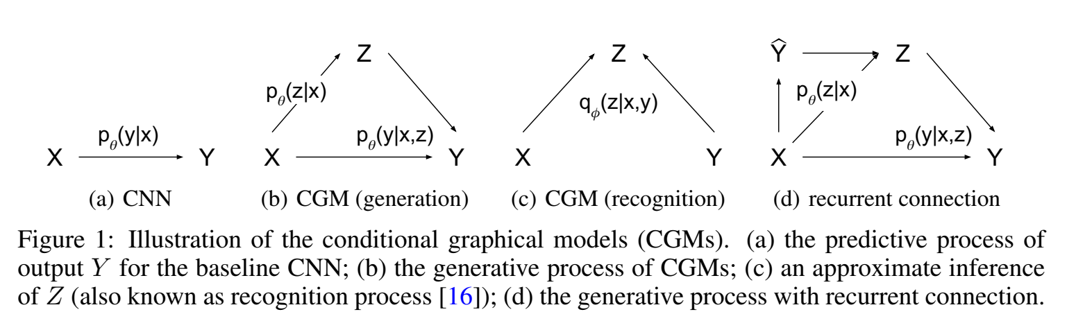
如下图所示 Fig1(a) 展示了x拟合y的分布,$p_\theta(y|x)$ ,Fig1(b)、Fig1(c)、Fig1(d)展示了三种conditional generative model (CGM) 。
Fig1(b) 是先验网络和生成网络、decoder,说的是x条件下生成z的真实分布,z和x共同作用生成y,我们输入给定的数据点x,由于生成z会有随机性,$p_\theta(y|x,z)$ 允许建模多种模式,因此生成的y也有随机性,y有很多种可能生成的样子,是一个one-to-many过程;
z的先验来自x,也可以放宽限制,把 $p_\theta(z)$ 写成 $p_\theta(z|x)$ 。
Fig1(c)是识别网络、encoder;
Deep CGMs 用 maximize the conditional log-likelihood训练,通常很难直接计算目标函数,因此也像VAE一样用SGVB框架(求导)训练。
variational lower bound of the model 写为:
$$
\log p_\theta(\mathbf{y} \mid \mathbf{x}) \geq-K L\left(q_\phi(\mathbf{z} \mid \mathbf{x}, \mathbf{y}) | p_\theta(\mathbf{z} \mid \mathbf{x})\right)+\mathbb{E}{q_\phi(\mathbf{z} \mid \mathbf{x}, \mathbf{y})}\left[\log p_\theta(\mathbf{y} \mid \mathbf{x}, \mathbf{z})\right]
$$
empirical lower bound 写为:
$$
\widetilde{\mathcal{L}}{\mathrm{CVAE}}(\mathbf{x}, \mathbf{y} ; \theta, \phi)=-K L\left(q_\phi(\mathbf{z} \mid \mathbf{x}, \mathbf{y}) | p_\theta(\mathbf{z} \mid \mathbf{x})\right)+\frac{1}{L} \sum_{l=1}^L \log p_\theta\left(\mathbf{y} \mid \mathbf{x}, \mathbf{z}^{(l)}\right)
$$
其中,$\mathbf{z}^{(l)}=g_\phi\left(\mathbf{x,y}, \epsilon^{(l)}\right), \epsilon^{(l)} \sim \mathcal{N}(\mathbf{0}, \mathbf{I})$ , $L$ 是样本数。
这种模型称为 conditional variational auto-encoder (CVAE) ,识别模型变成了 $q_\phi(z|x,y)$ ,生成模型变成了 $p_\theta (y|x,z)$ 。如Fig1(d)是一个CVAE结构,有一个循环结构,给定数据x,有一个初始预测的 $\hat y$ ,$q_\phi(z|x,\hat y)$ 采样出 z,再 $p_\theta (y|x,z)$ 生成 $y$ (重建)。
上式的推导过程为:
在条件VAE中,我们假设要建模的变量是 $y$ ,条件是 $x$ 。隐变量 $z$ 的近似分布 $q_\phi(z \mid x, y)$ 和真 实后验概率 $p_\theta(z \mid x, y)$ 之间的 KL-divergence 记为:
$$
\begin{aligned}
K L\left[q_\phi(z \mid x, y) | p_\theta(z \mid x, y)\right] &=\int q_\phi(z \mid x, y) \log \frac{q_\phi(z \mid x, y)}{p_\theta(z \mid x, y)} d \phi \
&=\int q_\phi(z \mid x, y) \log \frac{q_\phi(z \mid x, y) p_\theta(y \mid x) p_\theta(x)}{p_\theta(z, x, y)} d \phi
\end{aligned}
$$
展开:
$$
\begin{aligned}
& =\int q_\phi(z \mid x, y) \log _\phi(z \mid x, y) d \phi+\int q_\phi(z \mid x, y) \operatorname{logp}_\theta(y \mid x) d \phi+ \int q_\phi(z \mid x, y) \operatorname{logp}_\theta(x) d \phi -\int q_\phi(z \mid x, y) \operatorname{logp}_\theta(z, x, y) d \phi
\end{aligned}
$$
其中,第二项:
$$
\int q_\phi(z \mid x, y) \log p_\theta(y \mid x) d \phi=\log \theta(y \mid x)
$$
其余三项合并,原式
$$
K L\left[q_\phi(z \mid x, y)|| p_\theta(z \mid x, y)\right]=\log \theta(y \mid x)+\int q_\phi(z \mid x, y) \log \frac{q_\phi(z \mid x, y)}{p_\theta(y \mid x, z) p_\theta(z \mid x)} d \phi
$$
由于左侧 $K L \geq 0$ ,因此:
$$
\begin{aligned}
& \log \theta(y \mid x) \geq-\int q_\phi(z \mid x, y) \log \frac{q_\phi(z \mid x, y)}{p_\theta(y \mid x, z) p_\theta(z \mid x)} d \phi \
& =\mathbb{E}{q_\phi(z \mid x, y)}\left[\log p_\theta(y \mid x, z)+\log p_\theta(z \mid x)-q_\phi(z \mid x, y)\right] d \phi \
& =\mathbb{E}{q_\phi(z \mid x, y)}\left[\log \theta(y \mid x, z)\right]-\mathbb{E}{q_\phi(z \mid x, y)}\left[\log q_\phi(z \mid x, y)-\log \theta(z \mid x)\right] \
& =\mathbb{E}{q_\phi(z \mid x, y)}\left[\log \theta(y \mid x, z)\right]-K L\left[q_\phi(z \mid x, y)|| p_\theta(z \mid x)\right]
\end{aligned}
$$
左侧 $\log \theta(y \mid x)$ 是基于条件 $x$ 的后验概率,右侧是条件VAE的ELBO:
$$
E L B O=\mathbb{E}{q_\phi(z \mid x, y)}\left[\log p_\theta(y \mid x, z)\right]-K L\left[q_\phi(z \mid x, y) | p_\theta(z \mid x)\right]
$$
第一项是对隐变量 $z \sim p_\phi(z \mid x, y)$ 的期望下的极大似然估计,第二项是 $q_\phi$ 与先验的KL约束。同 样,第一项也要通过采样来估计,具体而言:
$$
\widetilde{\mathcal{L}}{\mathrm{CVAE}}(\mathbf{x}, \mathbf{y} ; \theta, \phi)=-K L\left(q_\phi(\mathbf{z} \mid \mathbf{x}, \mathbf{y}) | p_\theta(\mathbf{z} \mid \mathbf{x})\right)+\frac{1}{L} \sum{l=1}^L \log p_\theta\left(\mathbf{y} \mid \mathbf{x}, \mathbf{z}^{(l)}\right)
$$
Output inference and estimation of the conditional likelihood
推理的时候,评估模型预测准确度时,用z的期望(不采样z)作为样本z(不是直接采样一个z) $\mathbf{y}^*=\arg \max _{\mathbf{y}} p_\theta\left(\mathbf{y} \mid \mathbf{x}, \mathbf{z}^\right), \mathbf{z}^=\mathbb{E}[\mathbf{z} \mid \mathbf{x}] ^2$
计算这个期望可以用采样多个z的平均值,那么生成的样本变成 $\mathbf{y}^*=\arg \max {\mathbf{y}} \frac{1}{L} \sum{l=1}^L p_\theta\left(\mathbf{y} \mid \mathbf{x}, \mathbf{z}^{(l)}\right), \mathbf{z}^{(l)} \sim p_\theta(\mathbf{z} \mid \mathbf{x})$ 。
还有一种估计CGM的方法,是比较测试集的条件似然conditional likelihood,直接从prior network( $p_\theta(z|x)$ )里采样z个样本(这里z 的先验依赖于x),取似然平均,称为 Monte Carlo (MC) sampling :
$$
p_\theta(\mathbf{y} \mid \mathbf{x}) \approx \frac{1}{S} \sum_{s=1}^S p_\theta\left(\mathbf{y} \mid \mathbf{x}, \mathbf{z}^{(s)}\right), \quad \mathbf{z}^{(s)} \sim p_\theta(\mathbf{z} \mid \mathbf{x})
$$
但是这个方法需要样本数很多才准。因此作者提出用**重要性采样 **importance sampling 来估计条件似然:
这里impotance sampling原理是 $\mathbb{E}{p(a)}[\tau]=\mathbb{E}{p(b)}[\frac{p(a)}{p(b)}\tau]$
$$
p_\theta(\mathbf{y} \mid \mathbf{x}) \approx \frac{1}{S} \sum_{s=1}^S \frac{p_\theta\left(\mathbf{y} \mid \mathbf{x}, \mathbf{z}^{(s)}\right) p_\theta\left(\mathbf{z}^{(s)} \mid \mathbf{x}\right)}{q_\phi\left(\mathbf{z}^{(s)} \mid \mathbf{x}, \mathbf{y}\right)}, \quad \mathbf{z}^{(s)} \sim q_\phi(\mathbf{z} \mid \mathbf{x}, \mathbf{y})
$$
由上面的KL散度可知,$q_\phi(\mathbf{z} \mid \mathbf{x}, \mathbf{y})$ 和 $p_\theta(\mathbf{z} \mid \mathbf{x})$ 越接近越好,越接近说明采样的样本z更接近真实分布,可以用来衡量该样本对结果准确度的重要性。
Learning to predict structured output
用SGVB框架训练有个问题,就是训练时最优化了 $q_\phi(\mathbf{z} \mid \mathbf{x}, \mathbf{y})$ ,但是测试、推理时用的是 $p_\theta(\mathbf{z} \mid \mathbf{x})$ ,( 先验网络函数在训练里没有更新、$\theta$ 更新是通过生成网络 $p_\theta(y|x,z)$ 更新的 ),因此,可以在训练目标中加大KL散度项的权重,也就是让 $q_\phi(\mathbf{z} \mid \mathbf{x}, \mathbf{y})$ 和 $p_\theta(\mathbf{z} \mid \mathbf{x})$ 分布更接近,这样可以让训练和测试时隐变量z编码的差异没那么大。即 $-(1+\beta) K L\left(q_\phi(\mathbf{z} \mid \mathbf{x}, \mathbf{y}) | p_\theta(\mathbf{z} \mid \mathbf{x})\right)$ with $\beta \geq 0$。 加大权重虽然想法很好,但是在实验中发现没什么效果。
因此要找别的方法来减少训练和测试之间的差异,作者通过让 $q_\phi(\mathbf{z} \mid \mathbf{x}, \mathbf{y})=p_\theta(\mathbf{z} \mid \mathbf{x})$ ,也就是识别网络和预测网络用同一个网络。
则目标函数变成:
$$
\widetilde{\mathcal{L}}{\mathrm{GSNN}}(\mathbf{x}, \mathbf{y} ; \theta, \phi)=\frac{1}{L} \sum{l=1}^L \log p_\theta\left(\mathbf{y} \mid \mathbf{x}, \mathbf{z}^{(l)}\right), \text { where } \mathbf{z}^{(l)}=g_\theta\left(\mathbf{x}, \epsilon^{(l)}\right), \epsilon^{(l)} \sim \mathcal{N}(\mathbf{0}, \mathbf{I})
$$
称这种模型叫 Gaussian stochastic neural network (GSNN) 。结合CVAE和GSMN两种模型,就是两种都用,目标函数变成:
$$
\widetilde{\mathcal{L}}{hybrid}=\alpha\widetilde{\mathcal{L}}{CVAE}+(1-\alpha)\widetilde{\mathcal{L}}_{GSNN}
$$
CVAE for image segmentation and labeling
针对语义分割任务(属于 structured output prediction task )(语音分割应该是每个像素有某类语义),作者对于训练预测网络,提出两种训练方法:
- multi-scale prediction objective 多尺度预测目标(或者说output,预测出多个尺度的输出);
- structured input noise 结构化输入噪声;
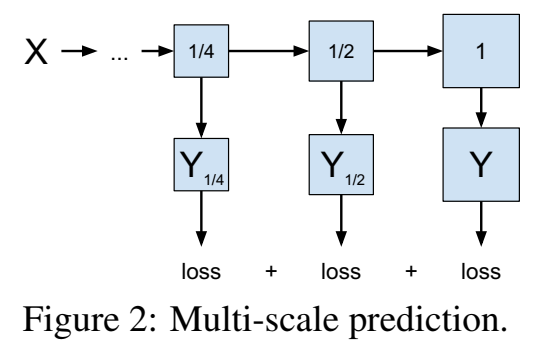
Training with multi-scale prediction objective
训练过程中,如下图所示,预测出原始输出的1/4、预测出原始输出的1/2、预测出原始输出,每个scale预测都有对应scale真实的重建误差。
比如要训练一张图片,一次前向传播中,就输出了1/4图片、1/2图片和整张图片。
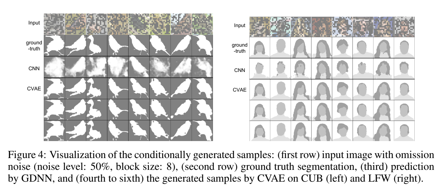
Training with input omission noise
给网络输入噪声是一种正则化方法,作者给输入input加噪,相当于给重建目标增加了难度。具体地,输入比如是图片,那么给输入图片随机一部分mask成0,相当于输入信息变少了(加噪了),给模型增加了难度,可以使得模型的泛化性变好。
Experiments
数据集 MNIST,任务是visual object segmentation and labeling 图像分割、图像标记。
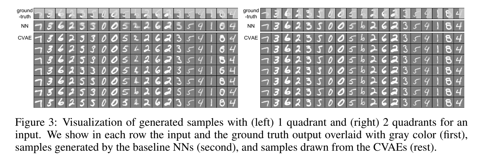
为了强调通过随机神经网络进行概率推断对于结构化输出变量的重要性,做了一个实验,是将图片分成四个象限,输入三个象限,让模型预测第四个象限、更大胆点,让模型预测更多的象限,随着模型要预测的东西越多(本来只要预测图片的一小部分,逐渐到要预测整张图片),生成的图片和输入图片就会越不同。
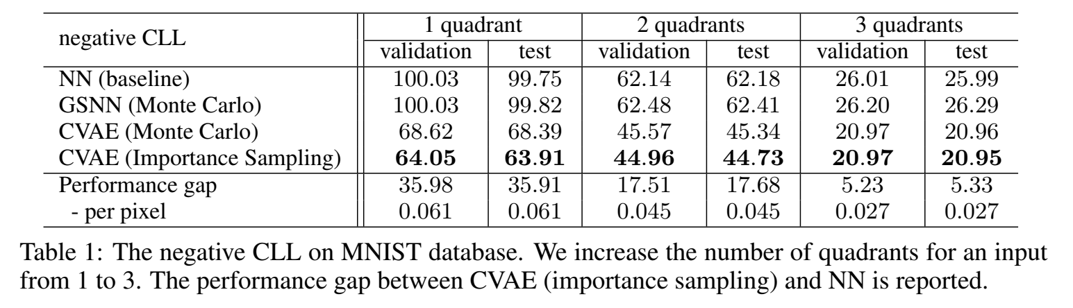
CVAE预测得更真实
Visual Object Segmentation and Labeling
todo
Object Segmentation with Partial Observations