GLOW
Kingma, Durk P., and Prafulla Dhariwal. “Glow: Generative flow with invertible 1x1 convolutions.” Advances in neural information processing systems 31 (2018). citations:1977 openai
github:https://github.com/openai/glow
【李宏毅深度学习】P59 Flow-based Generative Model
csdn :论文笔记(六)【Glow: Generative Flow with Invertible 1 x 1 Convolutions】
解决什么问题
生成高分辨率自然图像,以及其他生成任务;
用了什么方法
基于flow的生成方法,提出基于1×1卷积的flow方法,叫做glow;
效果如何
第一个可以有效生成高分辨率自然图像的基于似然的模型。
存在什么问题
生成质量不够高?
相关工作
生成模型的方法统称为likelihood-based method,可以分为三类:
- Autoregressive models 自回归模型,优点是简单,缺点是不能并行处理,计算量和输入长度成正比,不适用于输入长度很高的任务;
- Variational autoencoders(VAEs),目标是lower bound on the log-likelihoood of the data,可以并行,优化比较麻烦;
- Flow-based generative models 相比于前两种,有几个优点:
- Exact latent-variable inference and log-likelihood evaluation. 精确隐变量推断和对数似然估计。在VAE中,只能推断出与数据点对应的隐变量的近似值,而GAN没有encoder,不能进行latent的推断。由于flow-based model可逆,输出是一个精确值(而不是一个分布,再采样),优化目标也是数据的似然值,而不是lower bound。
- Efficient inference and efficient synthesis. 相比于自回归模型,flow在训练和生成过程都可以并行化。
- Useful latent space for downstream tasks.
- Significant potential for memory savings. 计算梯度的计算量在不同深度是constant,而不是linear;
背景:Flow-based Generative Models
对于一个不知道分布情况的数据,我们希望数据经过模型出来的概率值尽可能大,说明模型的输出分布接近数据分布。
数据x,x是高维任意向量,服从某个未知分布,模型输出 $p_\theta (x)$,数据集 $D$ ,log似然目标函数等于最小化:
- 对于离散变量 x:
$$
\mathcal{L}(\mathcal{D})=\frac{1}{N} \sum_{i=1}^N-\log p_{\boldsymbol{\theta}}\left(\mathbf{x}^{(i)}\right)
$$
- 对于连续变量 x:
$$
\mathcal{L}(\mathcal{D}) \simeq \frac{1}{N} \sum_{i=1}^N-\log p_{\boldsymbol{\theta}}\left(\tilde{\mathbf{x}}^{(i)}\right)+c
$$
其中 $\tilde{\mathbf{x}}^{(i)}=\mathbf{x}^{(i)}+u$ ,$u$ 是服从 $u \sim \mathcal{U}(0, a)$ 的均匀分布; $c=-M \cdot \log a$,$a$ 取决于数据的离散程度;$M$ 是 $\mathbf{x}$ 的维度;
对于大部分flow模型来说,生成过程可以定义为:
$$
\begin{array}{r}
\mathbf{z} \sim p_{\boldsymbol{\theta}}(\mathbf{z}) \
\end{array}
$$
$$
\mathbf{x}=\mathbf{g}_{\boldsymbol{\theta}}(\mathbf{z})
$$
其中,$\mathbf{z}$ 是latent variable,隐变量;$p_{\boldsymbol{\theta}}(\mathbf{z})$ 一个很简单、常见的密度函数,比如球形多高斯分布 $p_{\boldsymbol{\theta}}(\mathbf{z})=\mathcal{N}(\mathbf{z} ; 0, \mathbf{I})$ ;$\mathbf{g}_{\boldsymbol{\theta}}(..)$ 是可逆的,也被称为 bijective 双射(?),因此给一个数据点 $\mathbf{x}$ ,就可以推断出 隐变量 $z$,通过 $\mathbf{z}=\mathbf{f}\theta(\mathbf{x})=\mathbf{g}\theta^{-1}(\mathbf{x})$ ;为了简化,下面 $\mathrm{f}{\boldsymbol{\theta}}$ 和 $\mathbf{g}{\boldsymbol{\theta}}$ 的公式都省略 $\theta$;
$\mathbf{f}$ ($\mathbf{g}$ 也是)是由一系列transform组成的函数:$\mathbf{f}=\mathbf{f}_1 \circ \mathbf{f}_2 \circ \cdots \circ \mathbf{f}_K$ ,因此 $\mathbf{x}$ 和 $\mathbf{z}$ 之间的关系可以写为:
$$
\mathbf{x} \stackrel{\mathbf{f}_1}{\longleftrightarrow} \mathbf{h}_1 \stackrel{\mathbf{f}_2}{\longleftrightarrow} \mathbf{h}_2 \cdots \stackrel{\mathbf{f}_K}{\longleftrightarrow} \mathbf{z}
$$
这样的可逆变换序列也称为(归一化)流 flow。
通过变换下公式4,数据 $\mathbf{x}$ 的概率密度函数(pdf)可以写成:(参考李宏毅视频里的 $p_\theta (x)=p_\theta (z)|det(dz/dx)|$ )
$$
\begin{aligned}
\log p_{\boldsymbol{\theta}}(\mathbf{x}) &=\log p_{\boldsymbol{\theta}}(\mathbf{z})+\log |\operatorname{det}(d \mathbf{z} / d \mathbf{x})| \
&=\log p_{\boldsymbol{\theta}}(\mathbf{z})+\sum_{i=1}^K \log \left|\operatorname{det}\left(d \mathbf{h}i / d \mathbf{h}{i-1}\right)\right|
\end{aligned}
$$
其中,定义 $\mathbf{h}_0 \triangleq \mathbf{x}$ , $\mathbf{h}_K \triangleq \mathbf{z}$ , 标量值 $\log \left|\operatorname{det}\left(d \mathbf{h}i / d \mathbf{h}{i-1}\right)\right|$ 是 jacobian矩阵 $\left(d \mathbf{h}i / d \mathbf{h}{i-1}\right)$ 的行列式绝对值 取log,也叫 log-determinant;
思路是只选择那些 jacobian $d \mathbf{h}i / d \mathbf{h}{i-1}$ 是三角阵的transform,对于这些transform来说,log-determinant 就会很简单,可以写作:
$$
\log \left|\operatorname{det}\left(d \mathbf{h}i / d \mathbf{h}{i-1}\right)\right|=\operatorname{sum}\left(\log \left|\operatorname{diag}\left(d \mathbf{h}i / d \mathbf{h}{i-1}\right)\right|\right)
$$
其中,sum() 是所有vector元素求和,log()是element-wise log,diag()是jacobian矩阵的对角阵;
Glow
基于flow-based的生成模型,它没用之前flow-based模型中的生成器排列方式,在排列方式做了改进,用的1×1卷积;
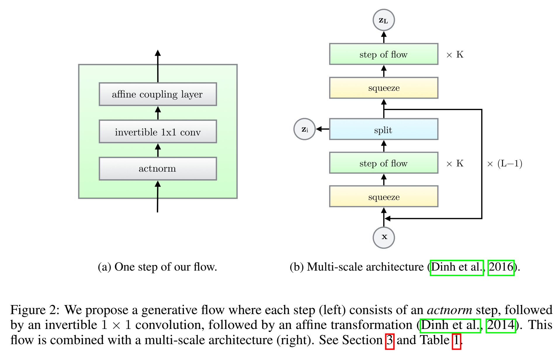
multi-scale architecture,结构包含actnorm 👉 invertible 1 × 1 convolution 👉 coupling layer ;
Actnorm: scale and bias layer with data dependent initialization
作用是normalization,但是用batch norm会不可逆,因此用activation norm;对每个channel进行缩放和bias(缩放和bias通过仿射变换实现),和BN一样有参数,初始化0均值单位方差;
an actnorm layer (for activation normalizaton), that performs an affine transformation of the activations using a scale and bias parameter per channel,
。。
Invertible 1 × 1 convolution
之前生成器堆叠都是固定的排列、堆叠顺序,这里提出一个代替固定排列的方法,是用参数可更新的可逆1×1卷积实现排列,并且这个排列不是固定的,因为里头的参数是会变化、会更新、会学习的。这里1×1卷积起到的作用打乱channel各个维度数据;
这里需要输入输出的channel数量一样。
输入是 $h \times w \times c$ 的tensor,卷积权重矩阵 $\mathbf{W}$ 是 $c \times c$ 的,则 可逆的 $1 \times 1$ convolution 的 log-determinant计算公式为:
$$
\log \left|\operatorname{det}\left(\frac{d \operatorname{conv} 2 \mathrm{D}(\mathbf{h} ; \mathbf{W})}{d \mathbf{h}}\right)\right|=h \cdot w \cdot \log |\operatorname{det}(\mathbf{W})|
$$
$\operatorname{det}(\mathbf{W})$ 的计算复杂度为 $\mathcal{O}\left(c^3\right)$, 而计算conv2D的复杂度为 $\mathcal{O}\left(h \cdot w \cdot c^2\right)$ ,初始化det为0?,收敛也是到0.
LU Decomposition
$\operatorname{det}(\mathbf{W})$ 的计算复杂度为 $\mathcal{O}\left(c^3\right)$ 可以通过LU分解减少到 $\mathcal{O}(c)$ :
$$
\mathbf{W}=\mathbf{P L}(\mathbf{U}+\operatorname{diag}(\mathbf{s}))
$$
其中 $\mathbf{P}$ is a permutation matrix, $\mathbf{L}$ 是对角线上有1的下三角矩阵, $\mathbf{U}$ 是一个对角线上为零的上三角矩阵, $\mathbf{s}$ 是一个 vector。
log-determinant公式简化为:
$$
\log |\operatorname{det}(\mathbf{W})|=\operatorname{sum}(\log |\mathbf{s}|)
$$
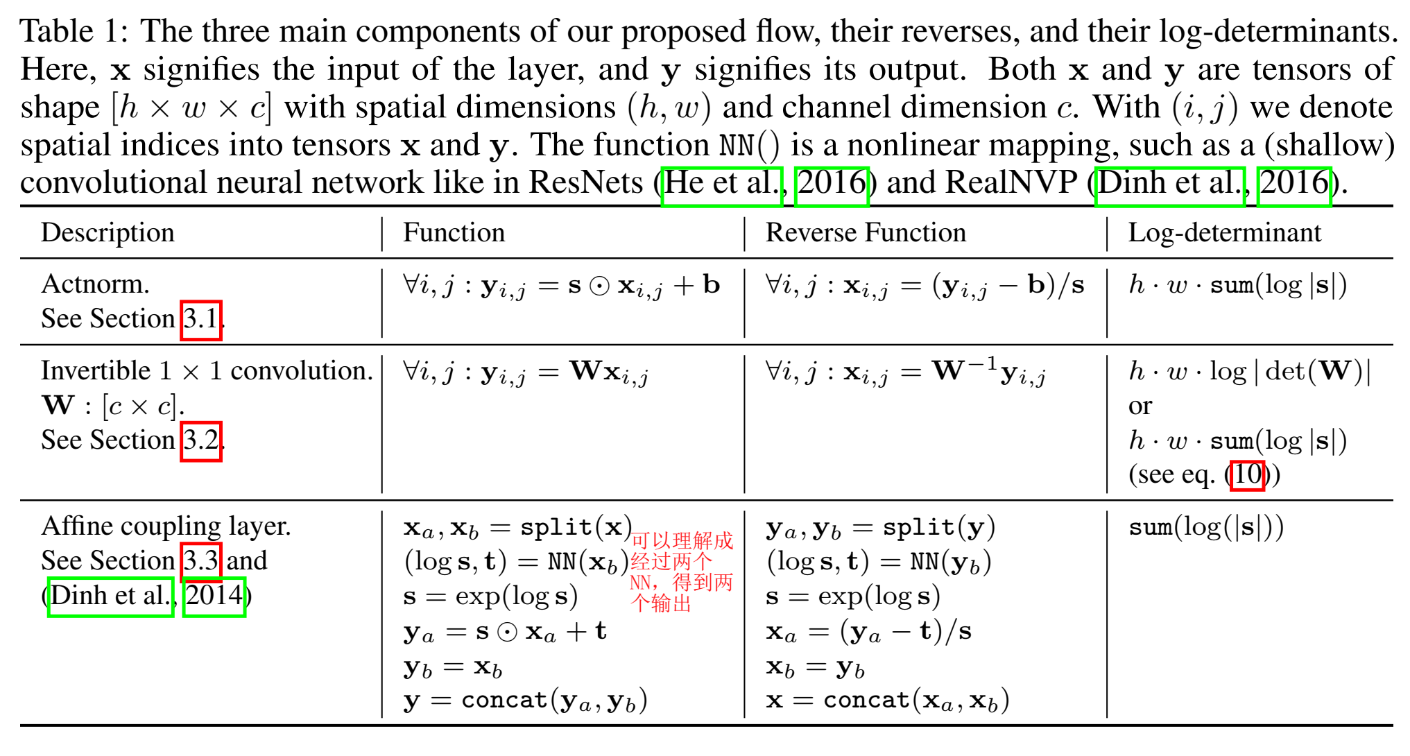
Affine Coupling Layers
下表列出了三个component的函数关系、逆函数的表达式,以及行列式的计算公式;(可参考李宏毅flow视频)
可以看出,行列式计算公式很简单,因此p(x)到p(z)关系很好求;
Related Work
基于IAF的MAF不能并行,自回归AR也不能并行,合成速度慢;GAN缺少latent-space encoders,输入不是特征x,并且优化困难;
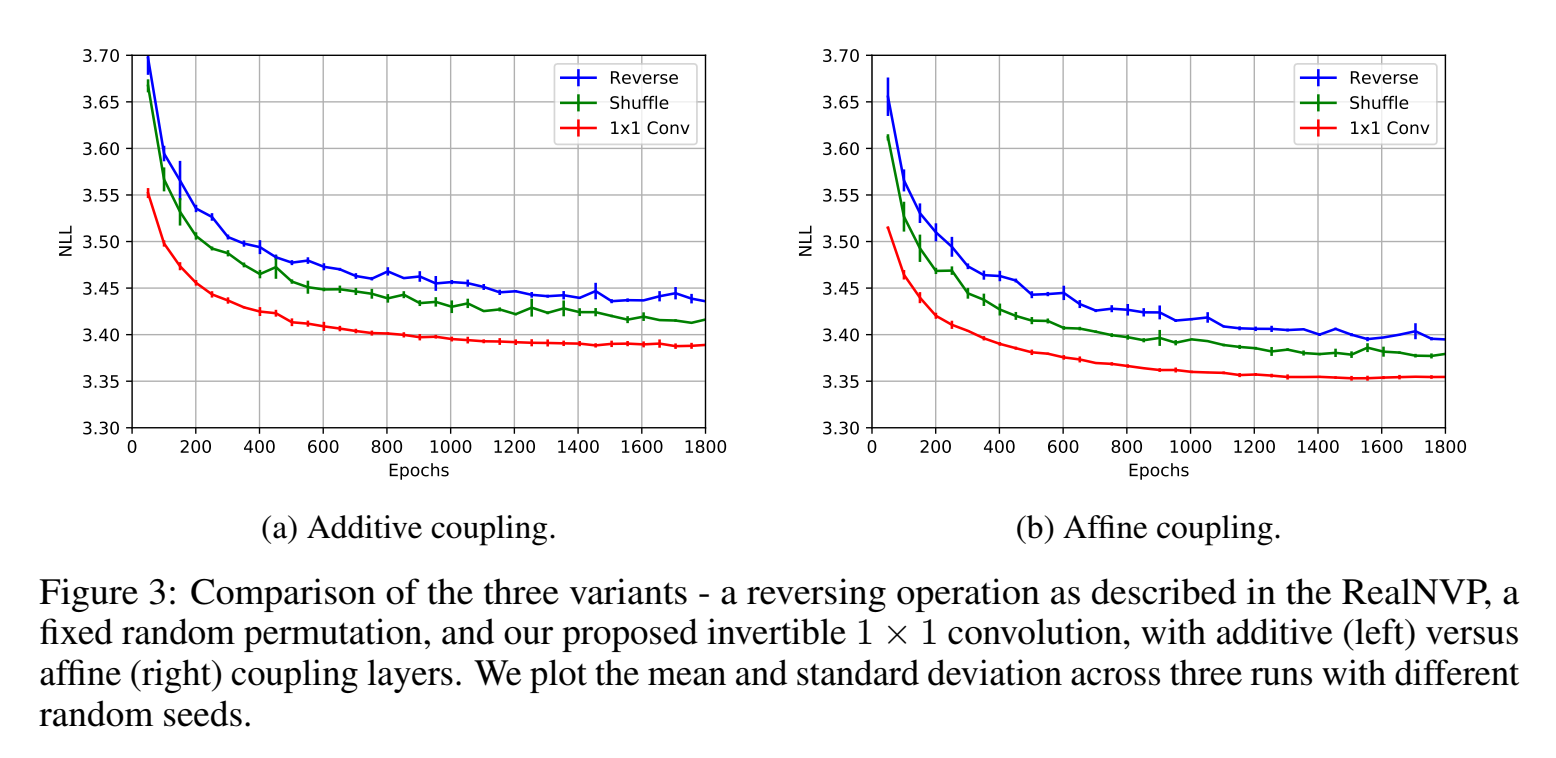
Quantitative Experiments
评价指标是平均负log似然 the average negative log-likelihood (bits per dimension) on the CIFAR-10 (越小越好)
Qualitative Experiments
todo
代码
Simple python implementation of the invertible 1 × 1 convolution
1 | # Invertible 1x1 conv |