使用Google Speech Commands dataset的论文

Google speech commands dataset：谷歌开源唤醒词数据集，有6万条，30个唤醒词，每条音频长度1s
Speech commands dataset v1 下载地址：http://download.tensorflow.org/data/speech_commands_v0.01.tar.gz
Speech commands dataset v2 下载地址：http://download.tensorflow.org/data/speech_commands_v0.02.tar.gz 或 https://storage.googleapis.com/download.tensorflow.org/data/speech_commands_v0.02.tar.gz
官方例子：https://www.tensorflow.org/tutorials/audio/simple_audio
输入t帧（其实就是1s），输出1个类别向量（每个类是一个关键词（yes、no、on、off……））

paper、code目录

Sainath, Tara N., and Carolina Parada. “Convolutional neural networks for small-footprint keyword spotting.” Sixteenth Annual Conference of the International Speech Communication Association. 2015

github开源代码：https://github.com/tensorflow/tensorflow/tree/master/tensorflow/examples/speech_commands

Choi S , Seo S , Shin B , et al. Temporal Convolution for Real-time Keyword Spotting on Mobile Devices[J]. 2019

github开源代码：https://github.com/hyperconnect/TC-ResNet

de Andrade, Douglas Coimbra, et al. “A neural attention model for speech command recognition.” arXiv preprint arXiv:1808.08929 (2018).

github开源代码：https://github.com/douglas125/SpeechCmdRecognition

Vygon, Roman, and Nikolay Mikhaylovskiy. “Learning efficient representations for keyword spotting with triplet loss.” International Conference on Speech and Computer. Springer, Cham, 2021

github：Github: Learning Efficient Representations for Keyword Spotting with Triplet Loss pytorch、nemo

Shan C, Zhang J, Wang Y, et al. Attention-based end-to-end models for small-footprint keyword spotting[J]. arXiv preprint arXiv:1803.10916, 2018.

github：https://github.com/isadrtdinov/kws-attention 网友的复现代码

github：https://github.com/Kirili4ik/kws-attention-pytorch 网友的复现代码

D. Seo, H. -S. Oh and Y. Jung, “Wav2KWS: Transfer Learning From Speech Representations for Keyword Spotting,” in IEEE Access, vol. 9, pp. 80682-80691, 2021, doi: 10.1109/ACCESS.2021.3078715.

github：https://github.com/qute012/Wav2Keyword

Howl: A Deployed, Open-Source Wake Word Detection System

github：https://github.com/castorini/howl pytorch

BYOL for Audio: Self-Supervised Learning for General-Purpose Audio Representation

github：https://github.com/nttcslab/byol-a pytorch

Stochastic Adaptive Neural Architecture Search for Keyword Spotting

github：https://github.com/TomVeniat/SANAS pytorch

Keyword Transformer: A Self-Attention Model for Keyword Spotting

github：https://github.com/ARM-software/keyword-transformer tensorflow

==Sainath, Tara N., and Carolina Parada. “Convolutional neural networks for small-footprint keyword spotting.” Sixteenth Annual Conference of the International Speech Communication Association. 2015. citation：383== 谷歌的论文

论文翻译：Convolutional Neural Networks for Small-footprint Keyword Spotting

开源代码，在TensorFlow官网可以下载

和Deep Kws做法一致，将DNN换成CNN
CNN输入：time*frequency，strides filters in frequency ，pools in time
尝试了不同下采样、pooling

==Shan C, Zhang J, Wang Y, et al. Attention-based end-to-end models for small-footprint keyword spotting[J]. arXiv preprint arXiv:1803.10916, 2018.==

github：https://github.com/isadrtdinov/kws-attention 网友的复现代码

github：https://github.com/Kirili4ik/kws-attention-pytorch 网友的复现代码

思想

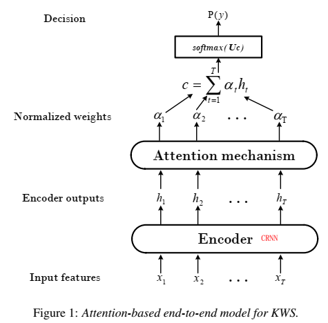
用attention机制的模型做命令词模型，没有事先训asr模型，输入T帧fbank语音特征，输出一个命令词概率，高于阈值就是命令词，是end2end，
用CRNN/GRU做encoder，输入fbank feature，输出high level feature（效果CRNN>GRU>LSTM）
CRNN性能好，但是有1.5s延时，还是GRU更合适。
attention用soft attention和average attention（效果soft attention>average attention）
减少计算量：滑动窗口时，每次滑动会得到一个T帧对应label概率，此时只要计算新添加的帧的计算，重叠部分不计算
运行时窗长都是100帧地执行，计算量小。[可改进之处]：当检测到keyword时（即当前帧超过给定的阈值，触发），那么就把窗长变为189帧，检测是否为keyword。
用20个滑动输出分类结果做smooth

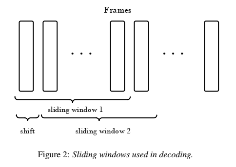
- 滑窗这个要好好想想怎么实现？答：雷博说：把倒一层构成c的每个α和h时间步的值都保留下来，然后下一帧来了，就可以只算下一帧的，然后再softmax计算。

实验

baseline用Deep KWS
网络结构：CRNN网络，一层CNN层，两层RNN层(64个节点)
训练集：正样本188.9k, 负样本 1007.4k
验证集：正样本9.9k, 负样本 53k
测试集：正样本 28.8k , 负样本32.8k
输入特征：PCEN特征。每条音频持续时间1.9 seconds.
four-syllable Mandarin Chinese term (“xiao-ai-tong-xue”) ，∼188.9K positive examples (∼99.8h) and ∼1007.4K negative examples (∼1581.8h) as the training set. 正样本：负样本=10：1

结果

∼84K parameters
1.02% FRR at 1.0 FA/hour.

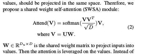
==Bai Y, Yi J, Tao J, et al. A Time Delay Neural Network with Shared Weight Self-Attention for Small-Footprint Keyword Spotting[C]//INTERSPEECH. 2019: 2190-2194==.

思想

用TDNN-attention结构做kws，输入音频特征，输出分类结果
特征量很小（12K）
没用RNN，用TDNN（前馈网络），减少计算量，支持并行
attention用的shared weight self-attention，就是Q、K、V本来由三个$w_ix+b_i$而来（不同project投影），现在是乘以同一个wx+b，最后是multi-head
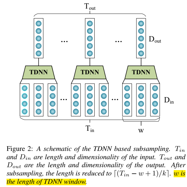
输入特征做下采样（tdnn povey原始论文也做的）
attention层后接两层tdnn，后接 global average
多帧输出->1个输出

模型结构为：

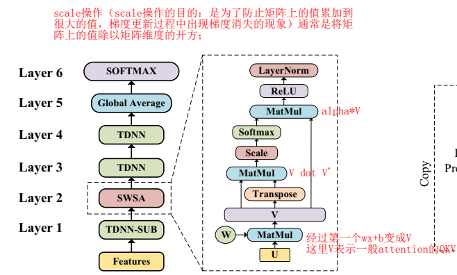
global average 做了polling，变成一个向量

最后softmax输出是只有一个向量

下采样为：

实验

数据集用Google Speech Commands ，都是1s，一个word的音频
10个命令词，20个filler（归为一个label）
用分类错误率作为评价指标

参考：A Time Delay Neural Network with Shared Weight Self-Attention for Small-Footprint Keyword Spotting浅析

中心思想：通过共享自注意力机制的权重，在维持性能不变的情况下，减少模型参数
本文的创新点：一是，用前馈神经网络代替在注意力机制中常用的回归神经网络，加速模型计算[用tdnn代替rnn]；二是，自注意力机制中的三个矩阵进行参数共享，减少模型参数
文章中提到的技术：TDNN、self-attention、SWSA(Shared-Weight Self-Attention)
TDNN技术：获取序列的局部特征
self-attention技术：用三个不同的权重矩阵将特征映射到不同空间中、获取序列的全局特征
shared-weight self-attention技术：用同一个权重矩阵将特征映射到同一空间中、减少模型参数。

模型结构：第一层TDNN-SUB（TDNN降采样层），实现方法：采用滑动窗的方式，在输入层矩阵Tin上设置一个宽度W为3（通常根据第一层拼帧结构决定）的滑动窗，当步长K超过1时（步长不易超过窗长），达到了降采样的效果，维度Dout减少为(Tin − w + 1)/k向上取整

第二层是SWSA（权重共享的自注意力机制），也是本文的重点，详细结构见F1（a）右手边虚框
第一步：输入为U，共享矩阵为W，Vi=WU，Vi为自注意力机制的输入，Vi是通过自注意力机制将输入特征U映射到某一空间得到的特征
第二步：由于权重共享，原来的Vq×Vk也就是现在的V×（V转置）即矩阵与矩阵本身点乘；
第三步：第二步得到的矩阵进行scale操作==（scale操作的目的：是为了防止矩阵上的值累加到很大的值，梯度更新过程中出现梯度消失的现象）通常是将矩阵上的值除以矩阵维度的开方==；
第四步：计算注意力得分，经过softmax层，对矩阵的每一行进行一个softmax规整，即矩阵的每一行的值加和为1；
第五步：将注意力得分与V点乘得到新的矩阵输出后紧跟RELU和LayerNorm层，最终得到SWSA层的输出
第三层和第四层是TDNN层
第五层：==globalAverage层：CNN中有类似的全局平均池化层==
在这边文章中未提及，但通过后面的实验章节推测，是权重矩阵每一列求平均值最终输出一个与当前层输入矩阵相同维度的向量

下面是权重共享后的self-attention公式：

multi-head self-attention版本

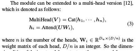
其中i的值等于共享权重矩阵的个数，当i为1是就是上述描述的权重共享self-attention机制；当i大于1是此时的共享权重是i个（类似于CNN有i个卷积核的概念），当i大于1时，权重矩阵的维度就会缩减为原来的1/i,通常为整数，其他步骤与上述的self-attention步骤一致，在self-attention输出层后增加一层将muli-head self-attention的输出拼接到一起，乘一个矩阵得到与i为1时相同大小的矩阵

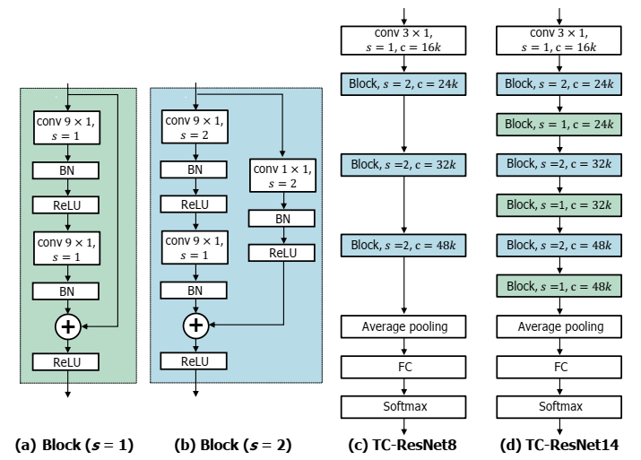
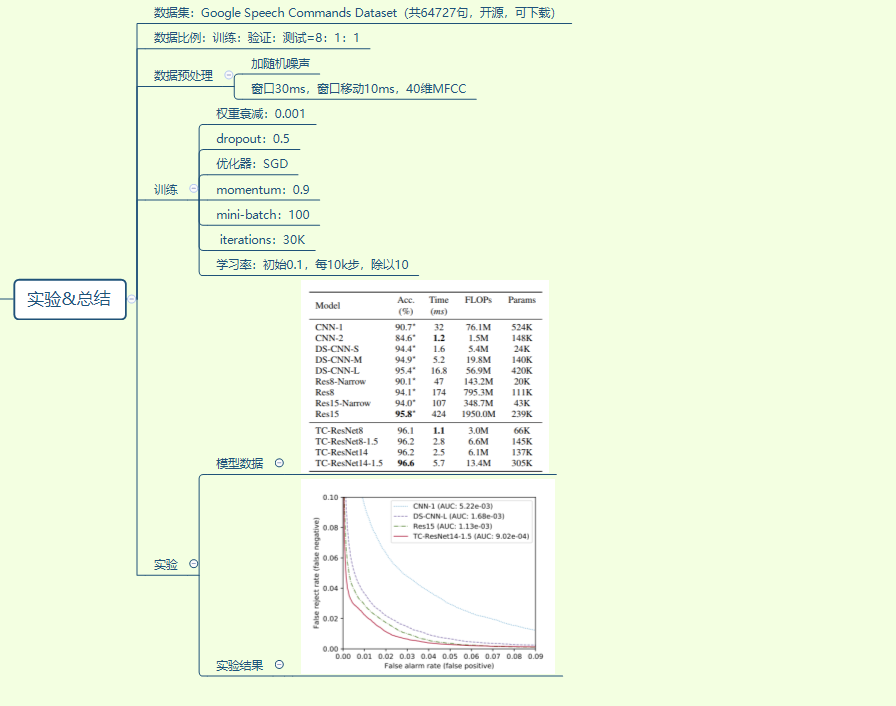
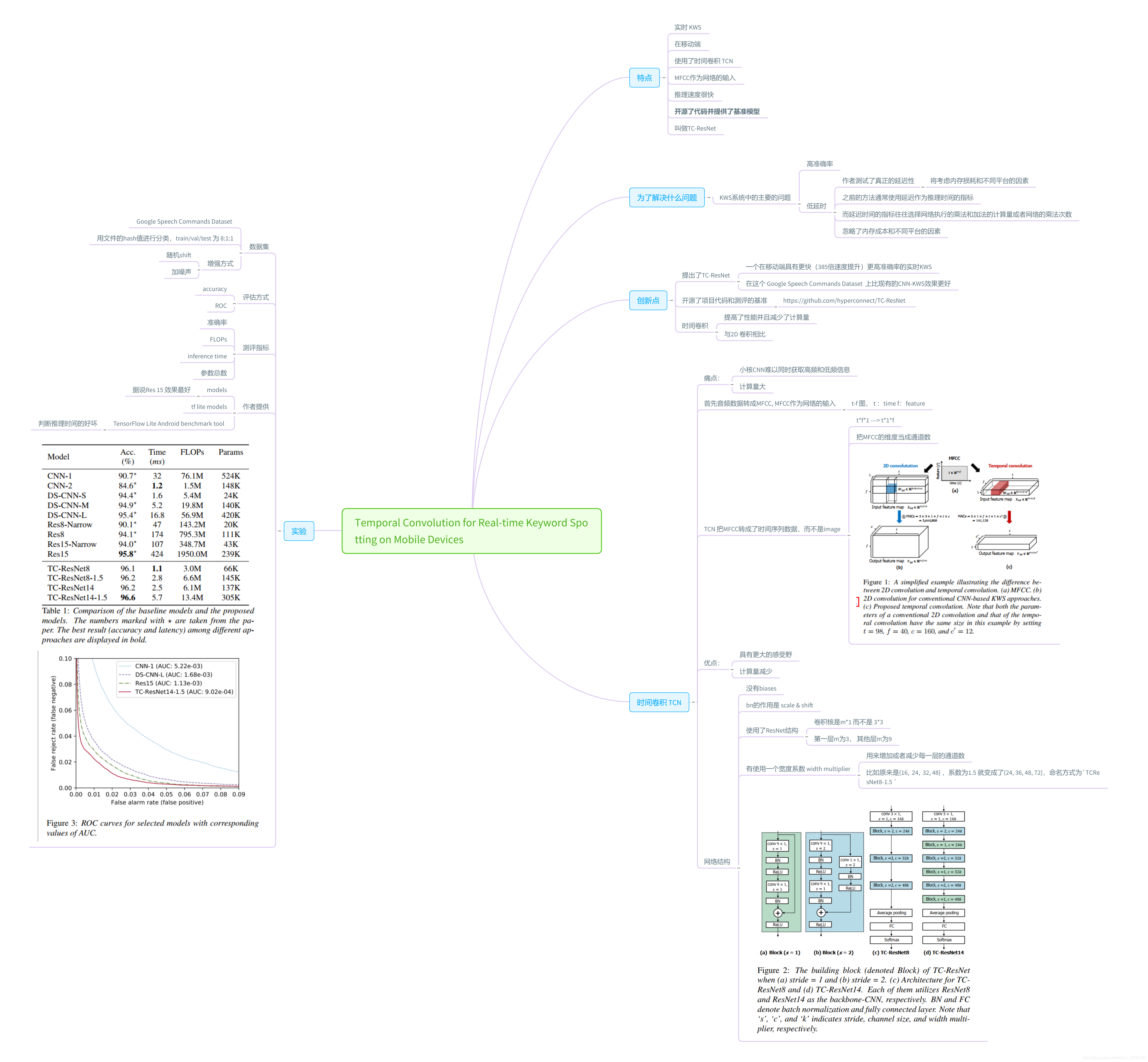
==Choi S , Seo S , Shin B , et al. Temporal Convolution for Real-time Keyword Spotting on Mobile Devices[J]. 2019. citation：41==

论文开源代码：https://github.com/hyperconnect/TC-ResNet

Lebhoryi的csdn笔记TC-ResNet

实时语音唤醒–Temporal Convolution for Real-time Keyword Spotting on Mobile Devices

思路

评测目标之一是测量在移动设备上的实际延迟 latency；
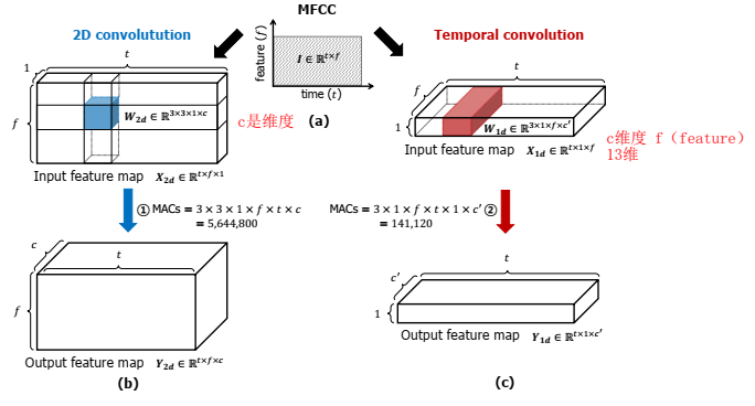
采用一维卷积，一维卷积优点：不对频率维度卷积，能具有更大的感受野（对于特征是语谱图输入的一些模型来说），同时获取高频和低频信息，计算量减少；

训练

输入MFCC，mfcc维度作为通道数c
使用一个宽度系数width multiplier，用来增加或减少每一层的通道数c，比如原来是{16,24,32,48}，乘1.5={24,36,48.72}，命名为TC-ResNet8-1.5
使用ResNet结构，cnn卷积核m *1（而不是3 *3），第一层m=3，其他层m=9
没有bias，bn层的作用是scale&shift
网络结构：（其中k是width multiplier倍乘系数）

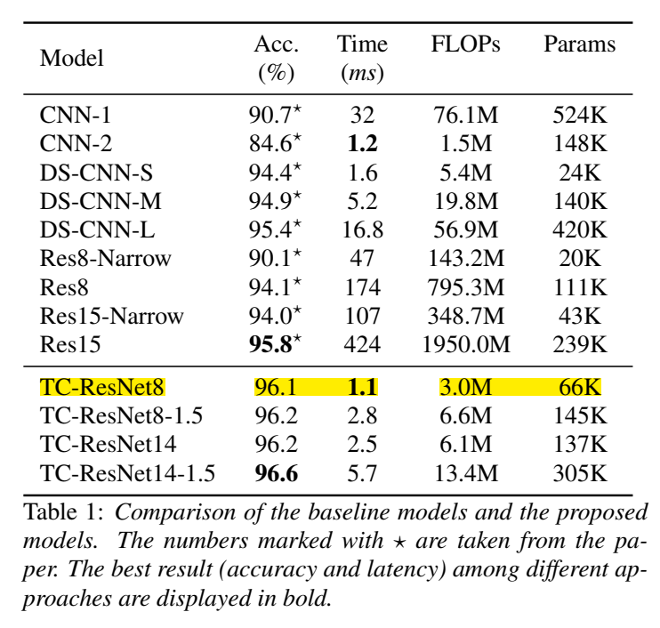
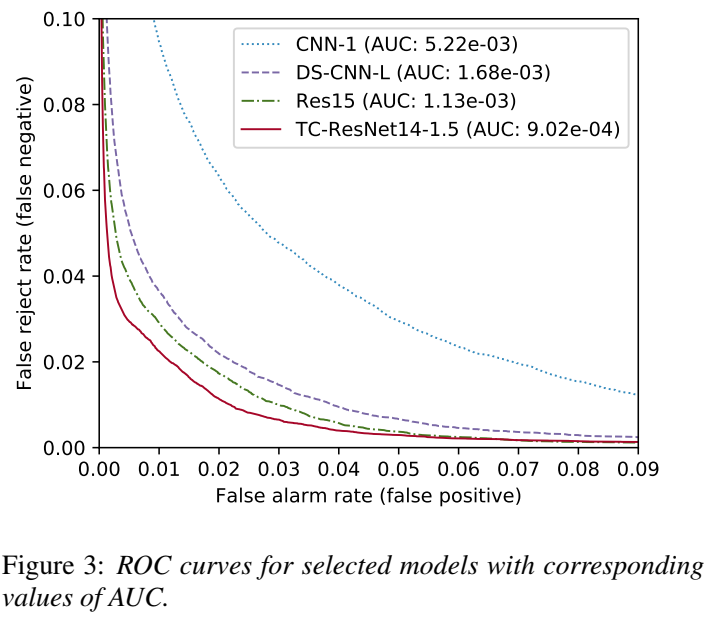
实验

实验结果考核了accuracy、ROC、耗时==FLOPs==、Params
TensorFlow Lite Android benchmark tool 判断推理时间的好坏

==Mittermaier S, Kürzinger L, Waschneck B, et al. Small-footprint keyword spotting on raw audio data with sinc-convolutions[C]//ICASSP 2020-2020 IEEE International Conference on Acoustics, Speech and Signal Processing (ICASSP). IEEE, 2020: 7454-7458. citation:14==

Lebhoryi的csdn笔记

思路

用SincNet直接读取原始音频进行训练

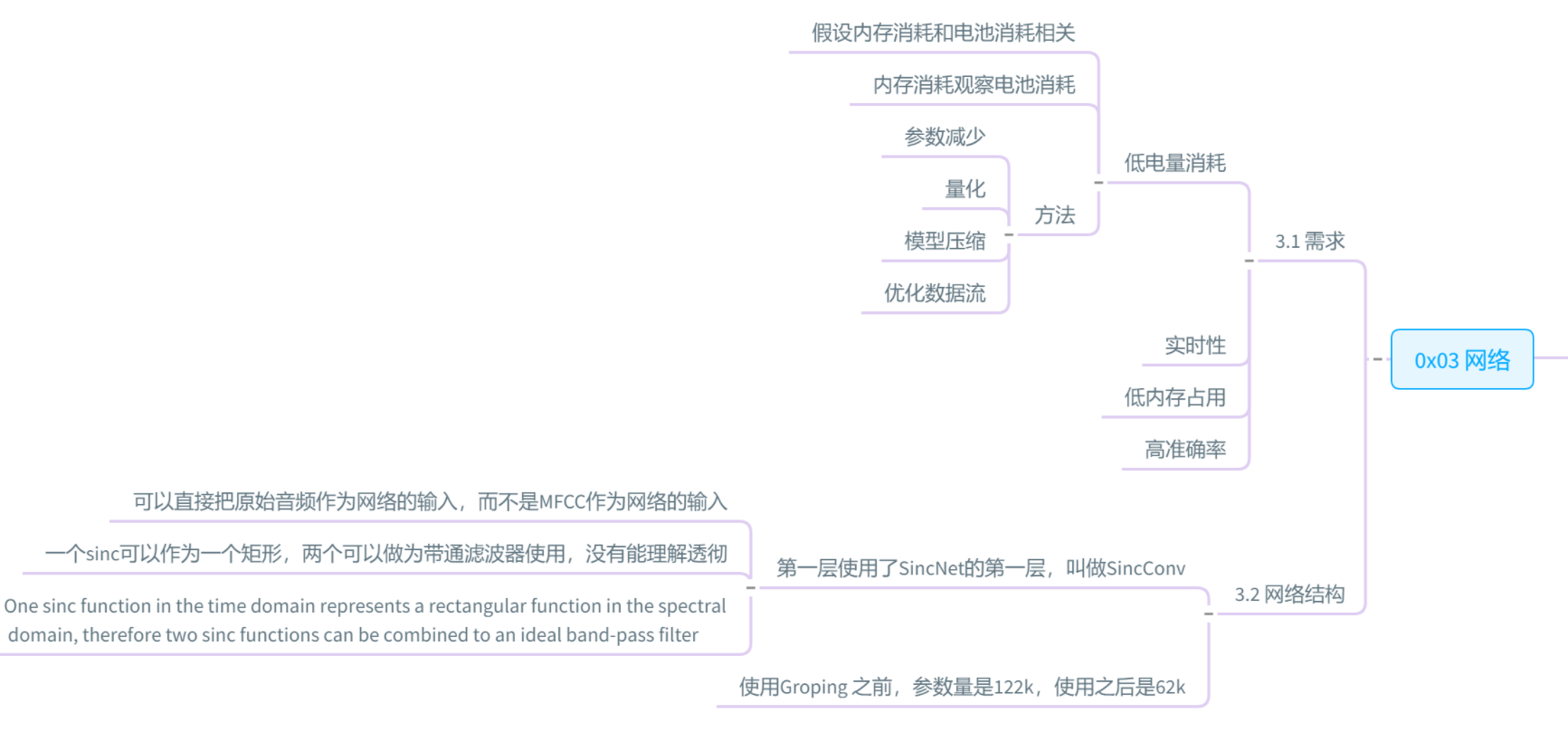
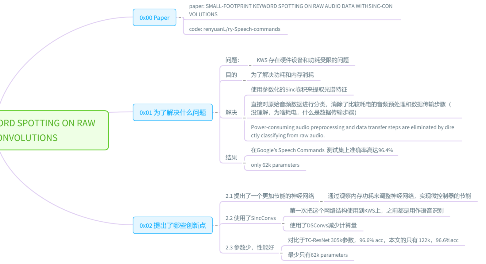
结果

sincConv+GDSConv模型的accuracy（97.3%）比TC-ResNet（96.6%）更高；参数量（62k）比TC-ResNet（305k）更少；

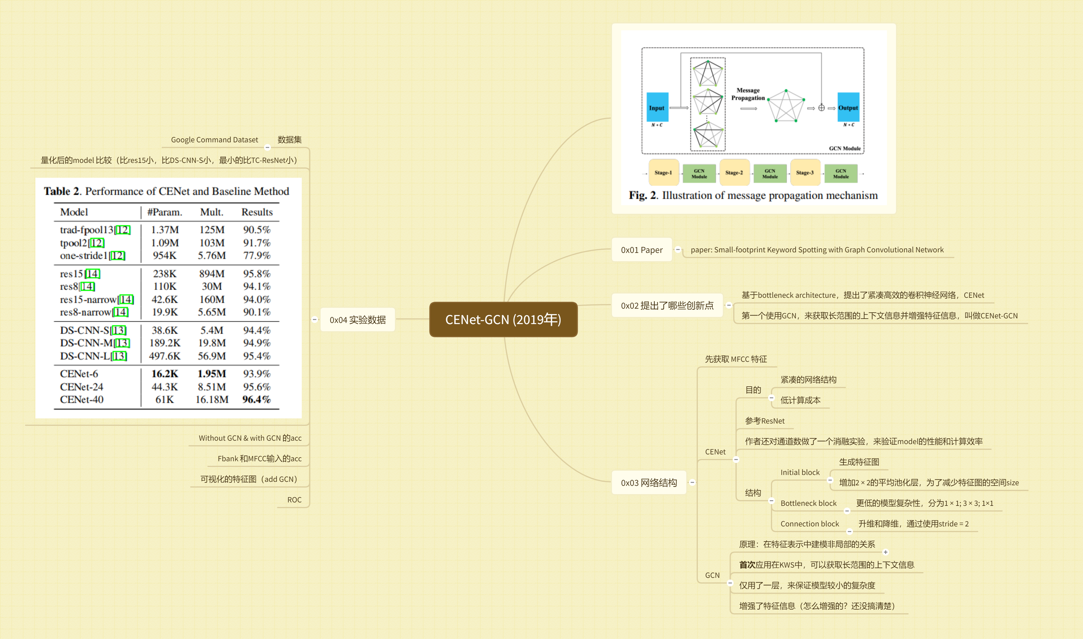
==Chen X, Yin S, Song D, et al. Small-footprint keyword spotting with graph convolutional network[C]//2019 IEEE Automatic Speech Recognition and Understanding Workshop (ASRU). IEEE, 2019: 539-546. citation：6==

Lebhoryi的csdn笔记CENet-GCN (2019年)

思路

使用了图神经网络GCN
结构紧凑

结果

【重要】

==Rybakov O, Kononenko N, Subrahmanya N, et al. Streaming keyword spotting on mobile devices[J]. arXiv preprint arXiv:2005.06720, 2020. citations：15== 谷歌的论文

github开源代码：https://github.com/google-research/google-research/tree/master/kws_streaming

Lebhoryi的csdn笔记stream_kws_cnn

思路

stream流式卷积也可以流式，意味着不用输入定长才有输出，输入任意一段（甚至只要给1帧）就会有输出，要研究代码，看是否可以一个vad长度输入，得到一个输出

A survey on structured discriminative spoken keywordspotting

==de Andrade, Douglas Coimbra, et al. “A neural attention model for speech command recognition.” arXiv preprint arXiv:1808.08929 (2018).==

github开源代码：https://github.com/douglas125/SpeechCmdRecognition

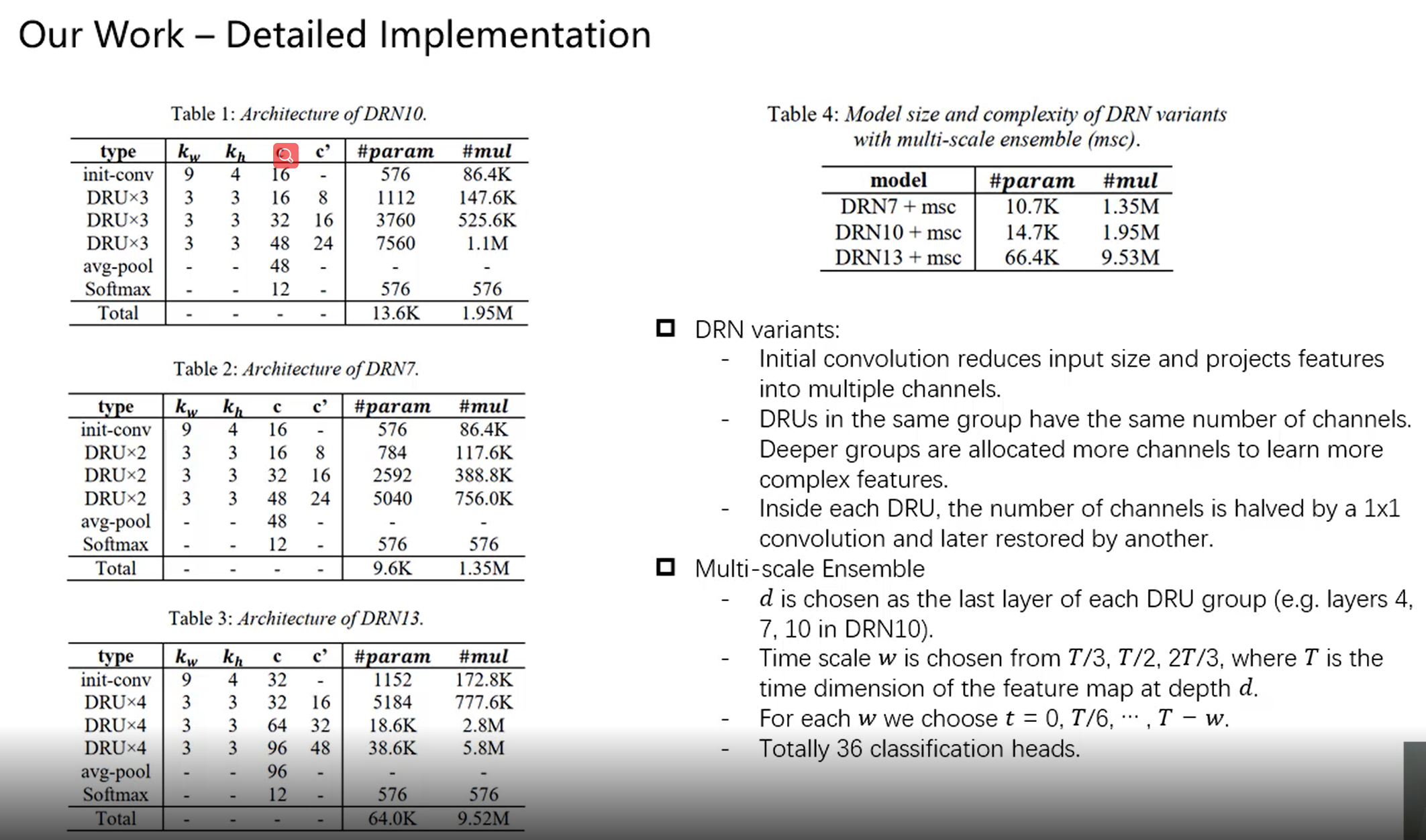
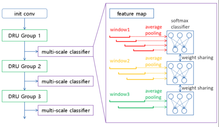
==Yang, Chen, Xue Wen, and Liming Song. “Multi-Scale Convolution for Robust Keyword Spotting.” INTERSPEECH. 2020.==三星研究院

线上会议video：http://www.interspeech2020.org/index.php?m=content&c=index&a=show&catid=321&id=835

PPT

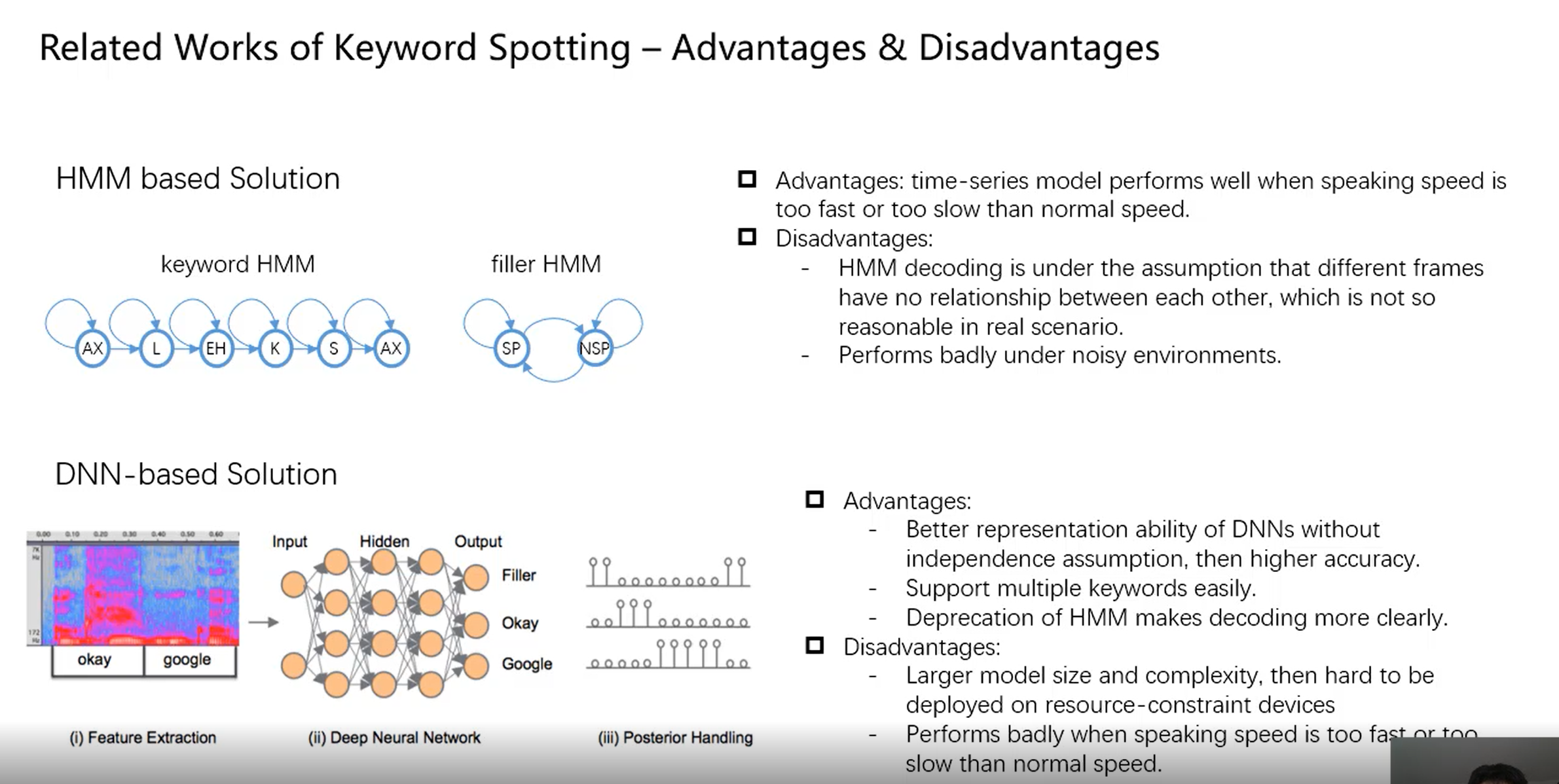
HMM在噪声环境下表现较差

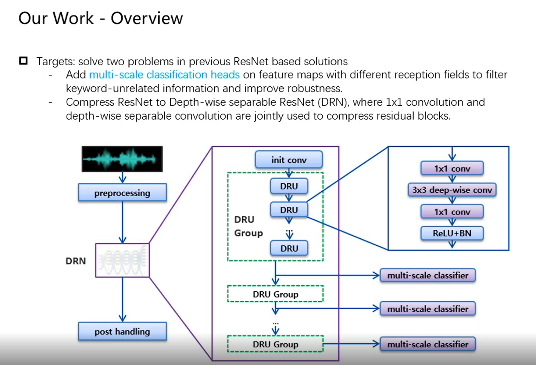
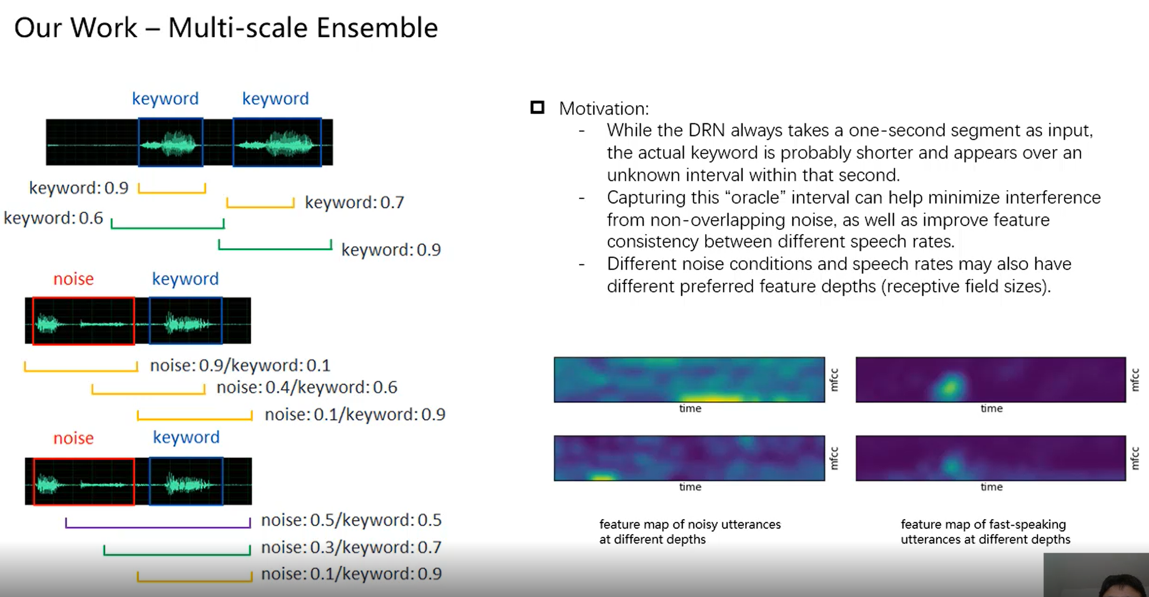
思路

实现低功耗small footprint：通过使用depthwise-separable convolutions in a ResNet framework；
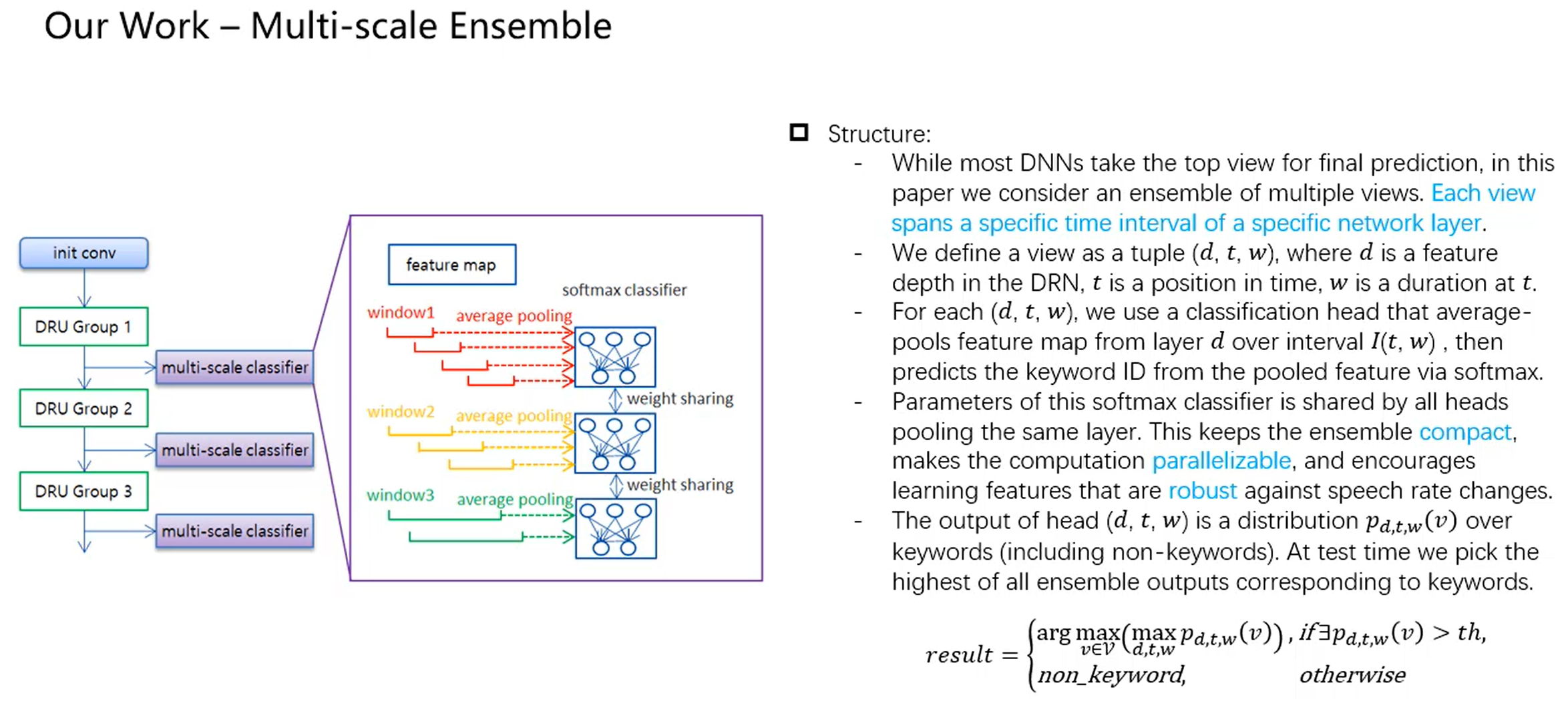
实现噪声鲁棒性：通过multi-scale ensemble of classifiers；每个分类器处理不同的输入特征，同时通过大量的参数共享让size紧凑；
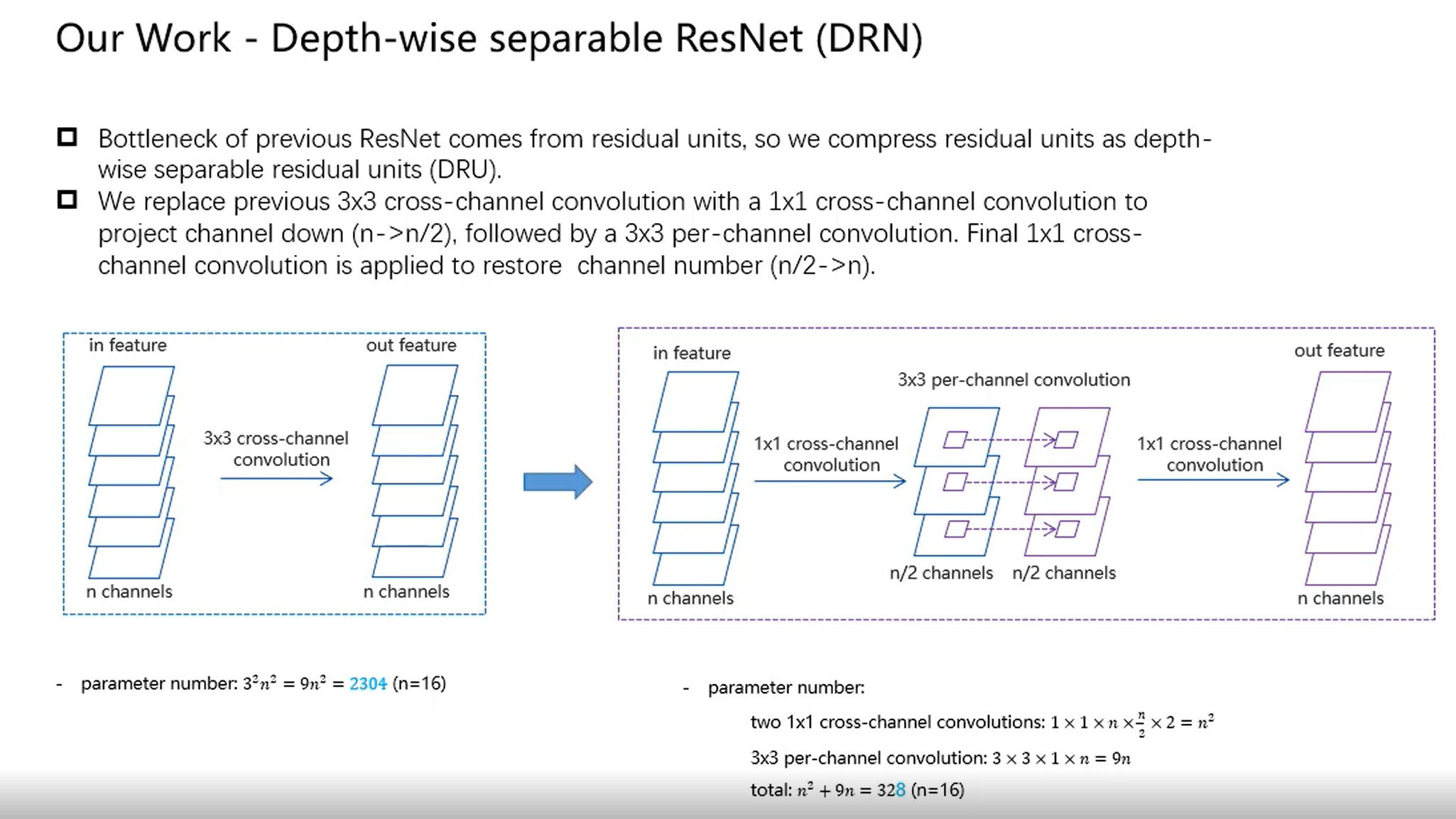
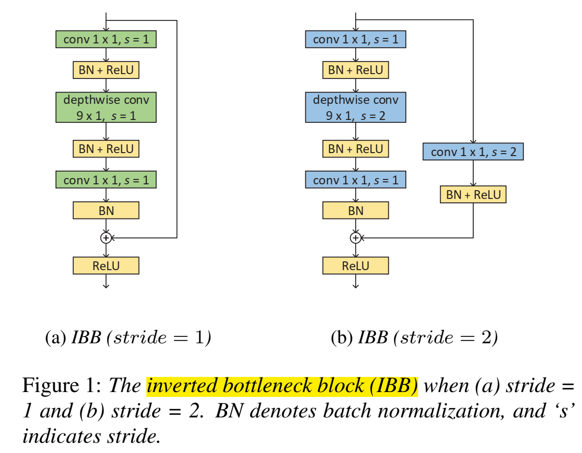
多个depthwise-separable residual unit (DRU) 堆叠起来的，用现在最流行的depthwise-separable cnn（减少参数量），然后加上resnet；
model compression in DRU 具体实现过程：Incoming 𝑛 -channel feature map is down-projected to 𝑛/2 channels by 1 × 1 convolution, processed per-channel by 3 × 3, up-projected to 𝑛 channels by another 1 × 1, then summed with original input to complete the residual unit；
1. 一开始正常1* 1卷积滤波器个数n/2，参数量 1* 1* n* n/2
2. 然后depthwise conv（channel个数n/2），参数量 3* 3* n/2
3. 最后1* 1 pointwise卷积（其实也是普通卷积）滤波器个数n，参数量 1* 1* n/2* n

Multi-scale ensemble 具体实现过程：

在不同的层，不同的t，不同的持续时间窗口w（d,t,w），抽取output，经过变换矩阵softmax，输出某个head的结果，每个head的帧取的时间间隔不同，比如第一个head是取0.8s，帧移0.4s取，第二个head是取1s，帧移0.5s取；

不同head所经过的变换矩阵里面的权重参数是一样的（经过同一个变换矩阵）（weight sharing），这是为了结构紧凑；

分类是数帧进行average pooling，再分类
loss function：$naiveCE:=\sum_{d,t,w}logp_{d,t,w}(y)$

分类判断 $ \large{result=\left{
\begin{aligned}
arg\max_{v\in{v}}(\max\limits_{d,t,w}p_{d,t,w}(v)),if{\exists}p_{d,t,w}(v)>th \
nonkeyword, otherwise
\end{aligned}
\right.}$

模型

10 conv layers in total, including one initial convolution and 9 stacked DRUs
Initial convolution reduces input size and projects features into multiple channels
The 9 DRUs are arranged in three groups. DRUs in the same group have the same number of channels. Deeper groups are allocated more channels to learn more complex features

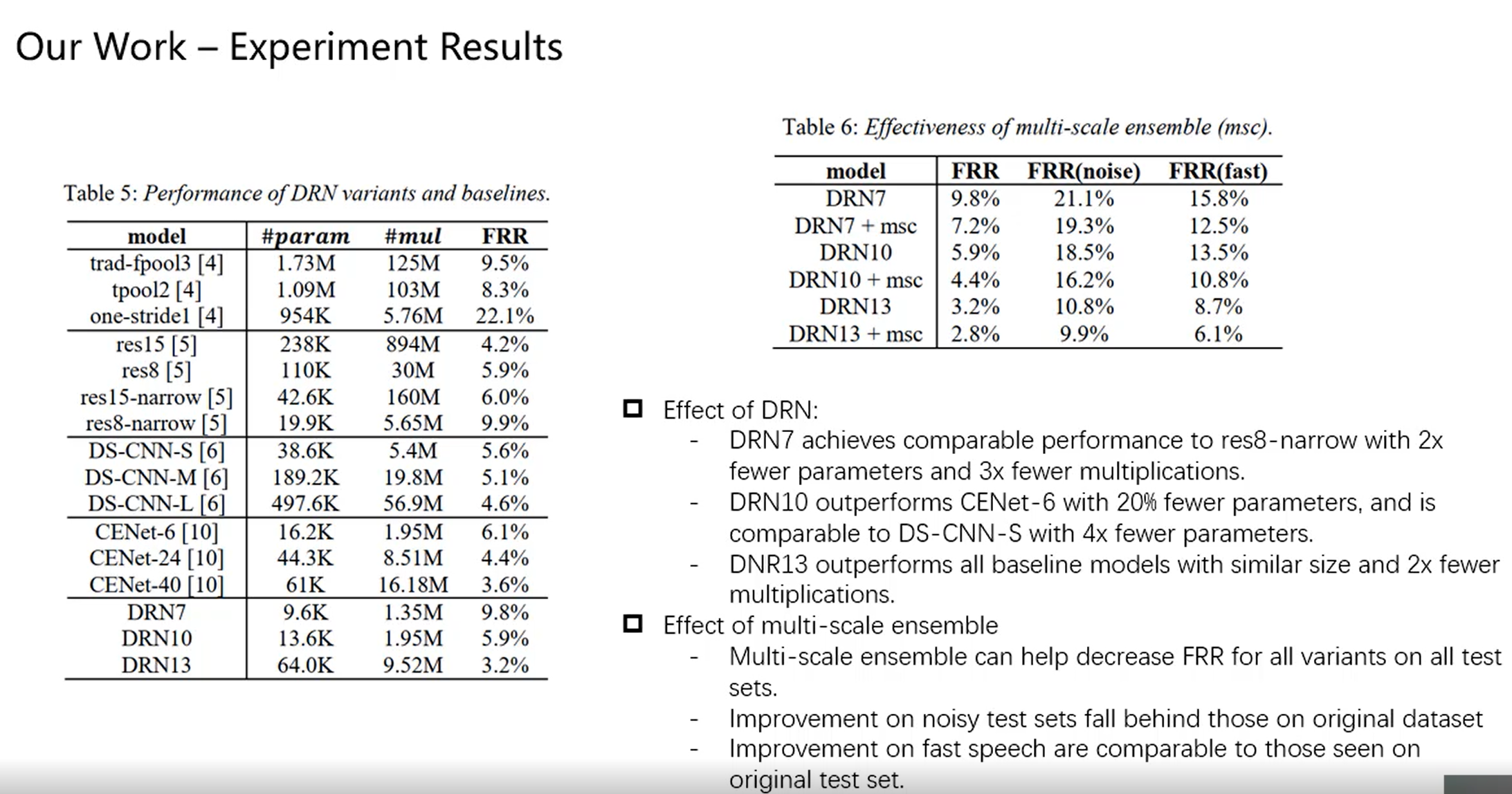
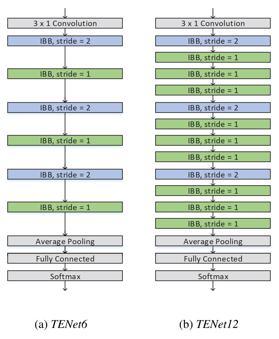
==Li, Ximin, Xiaodong Wei, and Xiaowei Qin. “Small-Footprint Keyword Spotting with Multi-Scale Temporal Convolution.” arXiv preprint arXiv:2010.09960 (2020).==

思路

一维卷积，time是长，没有宽，宽是1，特征维度（频率）是channel，这种卷积叫temporal convolution；
提出temporal efficient neural network (TENet) ，主要结构是inverted bottleneck block (IBB) ，该结构两头小中间大（和普通的bottleneck相反，因此叫inverted bottleneck），两头是1* 1卷积（沿着channel卷）（pointwise），中间是不沿着channel卷积的9*1卷积（depthwise），和普通的depthwise separable conv顺序相反。

IBB里的第一个1×1卷积的目的是通过扩展channel的数量，将input嵌入（embed）到高维子空间中；

IBB里的depthwise卷积是temporal卷积，通过对每个输入channel应用一个卷积滤波器，和非线性变换，来实现轻量级滤波；（注意这里只是depthwise conv不是depthwise seperate conv）

IBB里的最后一个1×1卷积将tensor转换回低维compact子空间，用于channels间的信息传输；

末尾层 average pooling -> fully connected -> softmax

提出Multi-branch Temporal Convolution Module，目的是为了捕捉短期和长期时间信息特征；

具体实现过程：让每个branch的kernel size都不同，从而帮助branch从它的时间粒度中学习不一样的模式；

多尺度融合（不同kernel size后的特征融合）：element-wise add（各个位置的元素等于两/N个输入矩阵相同位置元素的乘积的矩阵，再加和） (Hadamard product)

在训练时，将TENet中的所有depthwise卷积层都替换为MTConvs（IBB里独一个depthwise conv，替换成kernel size不同的多个depthwise conv（最后element-wise），叫做multi-scale））

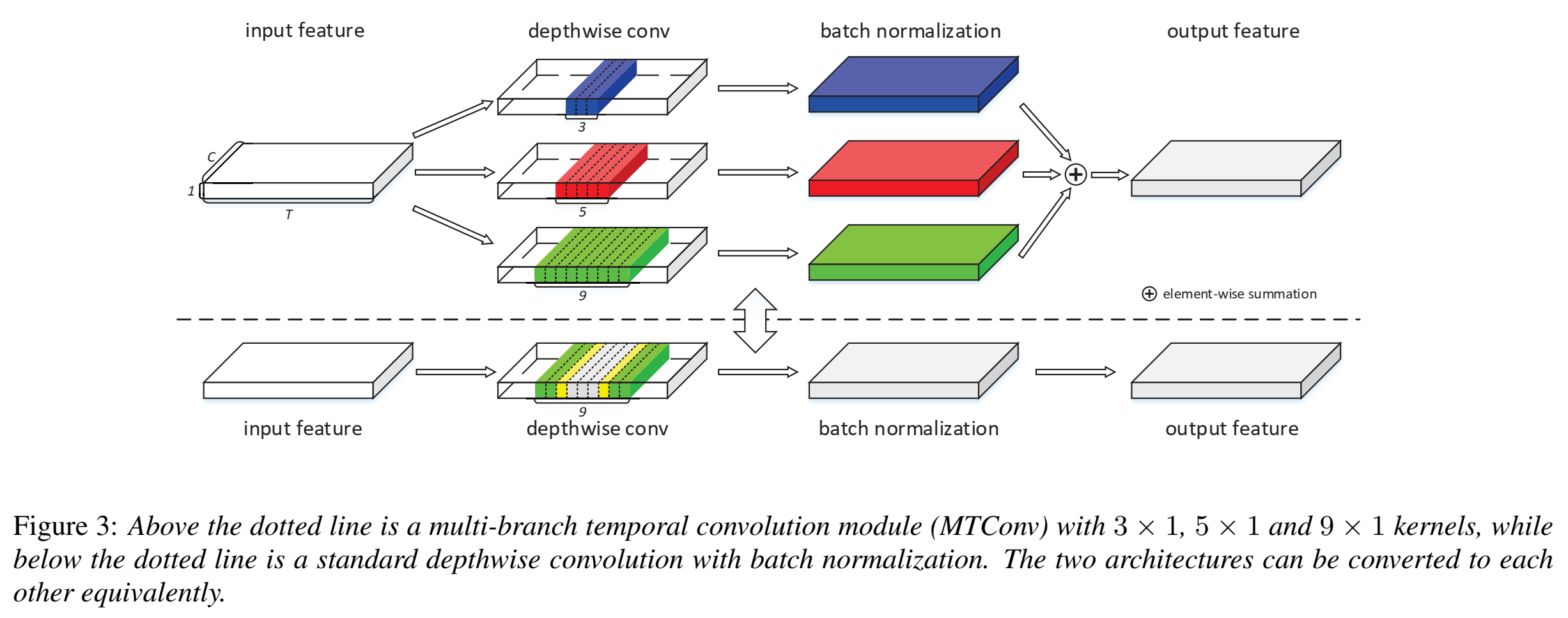
把下图原本只有一个的卷积，替换成多个不同kernel size卷积加和（上图）

kernel fusion of MTConv

$\large{O_{t,1,j}=(\sum\limits^k_{i=-k}M_{t+i,1,j}F_{i+k+1,1,j}-u_j)\frac{\gamma_j}{\sigma_j}+\beta_j}$

其中，M是输入，F是卷积核，$k=\frac{D-1}{2}$，D是卷积核尺寸（D×1×C），$u_j$和$\sigma_j$是BN层的channel-wise均值和标准差，$\gamma_j$和$\beta_j$是scaling和shifting系数（可训练更新）；

==Vygon, Roman, and Nikolay Mikhaylovskiy. “Learning efficient representations for keyword spotting with triplet loss.” International Conference on Speech and Computer. Springer, Cham, 2021.==ciations：12

github：Github: Learning Efficient Representations for Keyword Spotting with Triplet Loss

思路

triplet loss：$\large l(p_i,p_i ^+,p_i ^- = {0, g + D(f(p_i), f(p_i ^+)) - D(f(p_i), f(p_i ^-))})$

其中，$p_i$ 是anchor image，$p_i ^+$ 是positive image， $p_i ^-$ 是negative image，$g$ 是gap parameter regularizes the gap between the distance of the two image pairs: $(p_i,p_i ^+)$ and $(p_i,p_i ^-)$，D可以是欧氏距离；

这里是用来提embedding用的，输入A样本特征，输出embedding（高级特征），让A的embedding和同一个batch里的同类embedding距离近，让A的embedding和同一个batch里的不同类embedding距离远；

这里的triplet loss用来训练一个 triplet encoder
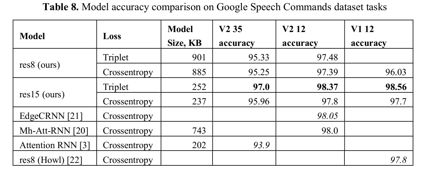
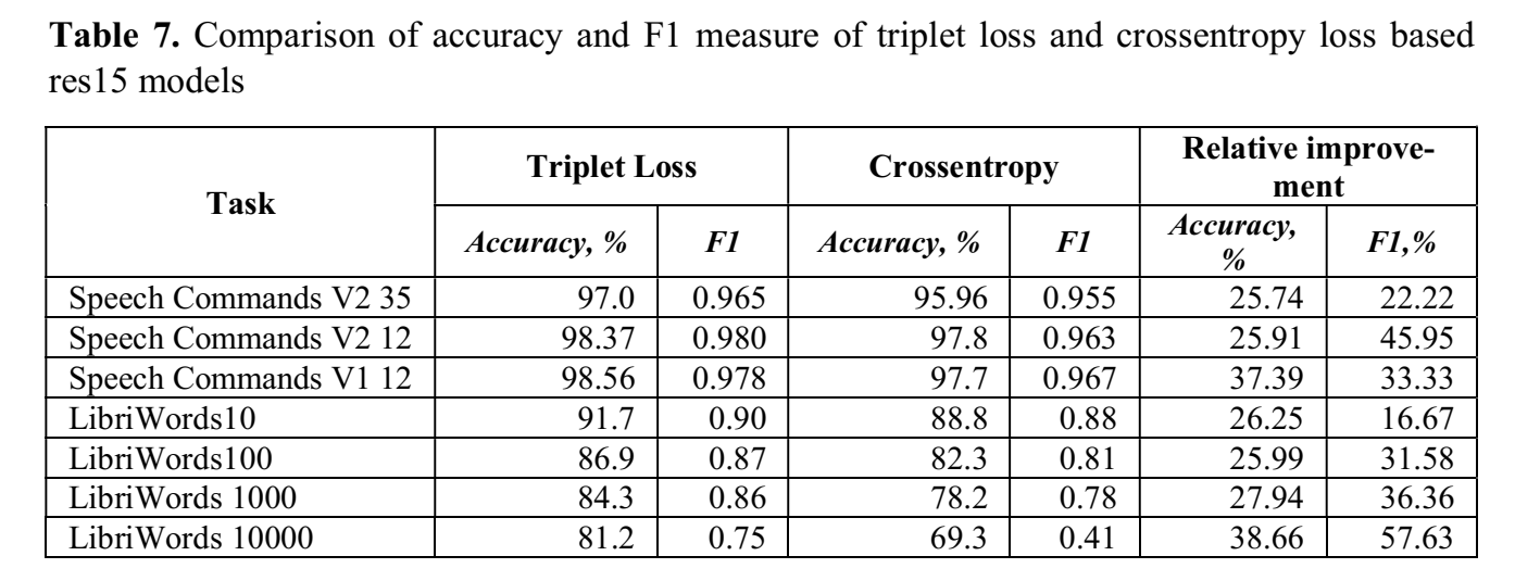
提出triplet-loss based metric embeddings + KNN分类器；实验优于ce，达到Google Speech Commands dataset 的SOTA（98.55% (V1 12分类(10keyword+sil+unknown)) 、98.37% (V2 12分类) ）；
提出基于音素相似度的batch sampling方法，改善了当数据不平衡时的F1
==论文中做实验表明RNN-based的模型用上triplet loss会变差==
先用模型提特征，把特征用KNN进行分类
batch sampling：Phonetic: Calculate a matrix of phonetic similarity for all the words in the dataset, sample batch_size/2 classes, then, for each sampled class add three random phonetically similar words (equally distributed) to the batch. Similarity score is calculated using SoundEx, Caverphone, Metaphone and NYSIIS algorithms；在一个batch里，相似的音多采样一点，triplet loss才比较有效，不然已经很不相似了，本身就很不像，不怎么需要区分开；

模型

基于Honk框架，直接用了（honk框架和wekws一样是框架），提高级特征（embedding）

实验

做了两组实验：

Google Speech Commands dataset；
LibriWords Datasets 这是用librispeech经过,the Montreal Forced Aligner(“Montreal forced aligner:Trainable text-speech alignment using kaldi” ) 对齐，得到word边界，进行实验，目的是查看用triplet loss在数据更大，分类数更多的情况效果能有多好；尝试了LibriWords10, LibriWords100, LibriWords1000, LibriWords10000

结果

代码

github：https://github.com/roman-vygon/triplet_loss_kws

requirement：安装nemo、nemo-asr、apex、protobuf==3.9.2，安装如下：

# 安装nemo
pip install nemo-toolkit[all]
pip install nemo_toolkit==0.10.1？
pip install nemo_toolkit[asr]？
# 安装protobuf：
pip install protobuf==3.9.2

# 安装apex 直接用pip install apex安装后会报错
git clone https://github.com/NVIDIA/apex
cd apex
pip install -v --disable-pip-version-check --no-cache-dir ./
#pip install -v --disable-pip-version-check --no-cache-dir --global-option="--cpp_ext" --global-option="--cuda_ext" ./

==Kim, Byeonggeun, et al. “Broadcasted residual learning for efficient keyword spotting.” arXiv preprint arXiv:2106.04140 (2021).==

github：/home/data/yelong/google-research/kws_streaming/models/bc_resnet.py

github网友复现代码：https://github.com/roman-vygon/BCResNet

思路

提出broadcasted residual learning方法、broadcasted-residual connection 、Broadcasting-residual network (BC-ResNet)

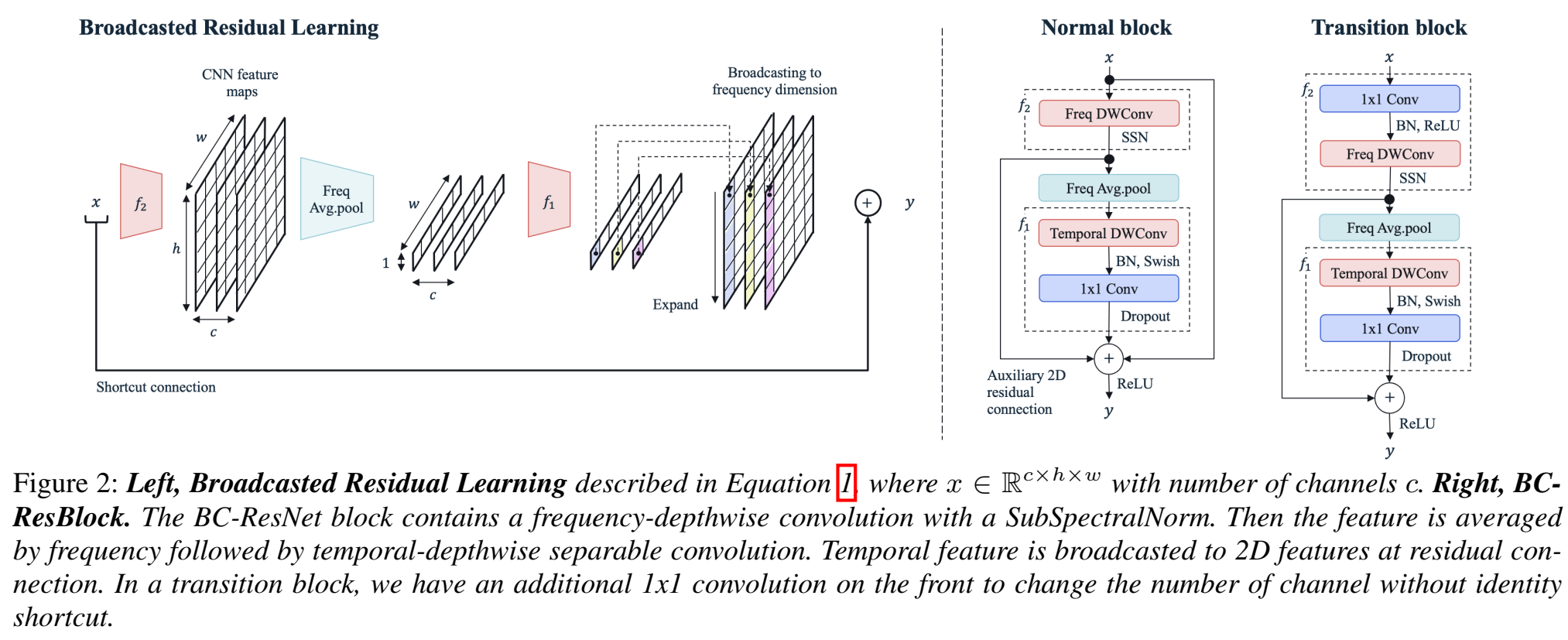
Broadcasted Residual Learning :在残差结构$y=x+f(x)$上改进为：$\large y=x+BC(f_1(avgpool(f_2(x))))$

其中，$f_1$是时间维度的函数，$f_2$是时间、频率二维图；

$f_2$ 输出也是二维的，然后对频率轴进行平均池化，得到时间、channel轴，再进入$f_1$函数，相当于$f_2$是一个提取不同帧时间/不同高低频率之间相关性的一个特征抽取器（我们之前拿frequency作为channel，这里是单独一个维度、（channel有它自己一个维度）），经过$f_1$后又扩展成2D；在每个residual block里重复这种平均、扩展操作；称之为Broadcasted Residual Learning
BC-ResNet Block ：$\large y=x+f_2(x)+ BC(f_1(avgpool(f_2(x))))$

流程：（描述时忽略channel通道）$x\in R^{h\times w}$ ,h是frequency，w是time，做3* 1的frequency-depthwise卷积（$f_2$），就是沿着频率h轴做depthwise卷积（滤波器数量和frequency一致，不求和，kerenl size=3），做SSN归一化，沿着频率轴做平均池化，再沿着时间轴w做1* 3time-depthwise卷积（$f_1$）（滤波器数量和time一致，不求和，kerenl size=3），接BN层，swish激活函数，再接1* 1 pointwise卷积，提取时间帧前后关系信息，再沿着channel轴做dropout，输出 $y\in R^{h\times w}$
SubSpectral Normalization (SSN) ：将输入频率分成多组，分别做归一化；用SSN代替BN层，来获取frequency-aware temporal features

12分类，训练时unknown和silence label的比例为10、10；40维mfcc 30ms帧长10ms帧移；time shift [-100,100]，概率0.8、0.8比例加噪、spec augment 只用two time 和two frequency masks，没用time wraping